FINITE ELEMENT ANALYSIS OF NOTCH-ROOT STRESS AND STRAIN CONCENTRATION FACTORS UNDER LARGE DEFORMATIONS Antonio Carlos de Oliveira Miranda Tecgraf – Computer Graphics Technology Group, Pontifical Catholic University of Rio de Janeiro, Rua Marquês de São Vicente 225, Rio de Janeiro, RJ, 22453-900, [email protected] Alexandre Lopes Tecgraf – Computer Graphics Technology Group, Pontifical Catholic University of Rio de Janeiro, Rua Marquês de São Vicente 225, Rio de Janeiro, RJ, 22453-900, [email protected] Marco Antonio Meggiolaro Dept. of Mechanical Engineering, Pontifical Catholic University of Rio de Janeiro, Rua Marquês de São Vicente 225, Rio de Janeiro, RJ, 22453-900, [email protected] Jaime Tupiassú Pinho de Castro Dept. of Mechanical Engineering, Pontifical Catholic University of Rio de Janeiro, Rua Marquês de São Vicente 225, Rio de Janeiro, RJ, 22453-900, [email protected] Luiz Fernando Martha Dept. of Civil Engineering, Pontifical Catholic University of Rio de Janeiro, Rua Marquês de São Vicente 225, Rio de Janeiro, RJ, 22453-900, Brazil, [email protected] Abstract: There is a vast literature on linear-elastic stress concentration factors Kt (Peterson, 1997), which depend solely on the specimen/notch geometry and on the type of loading. However, in the presence of plasticity at the notch root, the actual stress concentration factor Kσ is found to be smaller than the tabulated Kt, mainly due to the stress redistribution at the yielding zone. In turn, the strain concentration factor Kε at the notch root, which strongly affects the fatigue life predicted by the εN method, can be much larger than Kt. Several models have been proposed to assess the elastic-plastic behavior at the notch root, such as the rules proposed by Neuber (1961), Glinka (1985), Topper et al. (1969), Seeger et al. (1980), and Hoffman et al. (1985). In many cases, these models may provide reasonable estimates of the maximum stresses and strains at the notch root; however, the differences among the fatigue life predictions by each rule can be unacceptably large. In addition, these methods do not account for the geometrical changes at the notch root under large displacements, leading to further errors. In this work, 2D finite element analyses are carried out to evaluate elastic-plastic stress and strain distributions ahead of a notch under large deformations, at several load levels. Based on this analysis, the main strain concentration rules proposed in the literature are evaluated and their applicability verified. In particular, it is verified that Neuber’s rule is able to predict reasonable estimates of the concentration factors, as long as both nominal and notch-root stresses are modeled as elastic-plastic, as stated by Meggiolaro et al. (2002). It is concluded that several claims of Neuber’s underestimation of Kσ and overestimation of Kε are in fact a product of inappropriate simplifications in the material modeling and high sensitivity to the inherent finite element calculation errors. Keywords: Stress concentration, notch root, elastic-plastic analysis, finite elements.

1. INTRODUCTION The εN is a modern fatigue design method (Dowling, 1993; Fuchs and Stephens, 1980; Rice, 1988; Sandor, 1972) in which Neuber is the most used equation to correlate the nominal stress σn and strain εn ranges with the stress σ and strain ε ranges they induce at a notch root. The Neuber equation states that the product between the stress concentration factor Kσ (defined as σ/σn) and the strain concentration factor Kε (defined as ε/εn) is constant and equal to the square of the geometric stress concentration factor Kt, thus K t2 =

σ⋅ε σn ⋅ εn

(1)

Some authors prefer to use Kf, the fatigue concentration factor, instead of Kt in this equation (Topper et al., 1969). When the nominal stresses are lower than SYc, the cyclic yielding strength, it is common practice to model them as Hookean and, therefore, to use the Neuber equation in the simplified form: K t2 =

σ⋅ε⋅E

(2)

σ n2

Ramberg-Osgood is one of many empirical relations that can be used to model the cyclic response of the materials. Its main limitation is to not recognize a purely elastic behavior, and its main advantage is its mathematical simplicity. It can be used to describe the stresses and strains at the notch root by σ ⎛ σ ⎞ ⎟ ε = + ⎜⎜ E ⎝ H c ⎟⎠

1 / hc

(3)

in which E is the Young’s modulus, Hc is the hardening coefficient and hc is the hardening exponent of the cyclically stabilized σε curve. Eliminating ∆ε from Equations (2) and (3), σn is directly related to ∆σ by K t2 σ n2 = σ 2 +

Eσ (hc +1)/ h c ( H c )1/ h c

(4)

However, the above equation is logically incongruent, since it treats the very same material by two different constitutive models: Ramberg-Osgood at the notch root and Hooke at the nominal region. Moreover, this procedure can generate significant numerical errors even when the nominal stresses are much lower than the material cyclic yielding strength, as it will be discussed next. 2. LIMITATIONS OF THE SIMPLIFIED NEUBER APPROACH To avoid the errors induced by the simplified (Hookean) Neuber approach, it is necessary to use the Ramberg-Osgood model to describe not only the stresses at the notch root, but also to describe the nominal stresses, writing ⎛σ ⎞ σ ε n = n + ⎜⎜ n ⎟⎟ E ⎝ Hc ⎠

1 / hc

(5)

In this case, given the nominal stress range ∆σn, the stress range at the notch root ∆σ can be calculated from Equations (1), (3), and (5), yielding K t2 ( σ n2 +

E σ n(hc +1)/ hc ( H c ) 1/ h c

) = σ 2+

Eσ (h c +1)/ h c

(6)

( H c ) 1/ h c

stress and strain concentration factors

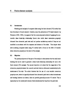
Figure (1) shows a comparison between the stress Kσ and strain Kε concentration factors predictions made by the simplified Neuber approach using Equation (4), and the general (corrected) ones obtained using Equation (6), for a SAE 1009 steel when the notch root has a Kt of 3. As it can be seen in the figure, for nominal stress amplitudes σn smaller than 0.5⋅SYc both predictions result in roughly the same concentration factors. However, for larger nominal stress values the predictions diverge, and the classical Neuber approach wrongfully predicts ever increasing strain concentration factors Kε and even stress concentration factors Kσ smaller than unity, a complete non-sense. 10 8

classical Neuber approach

6 Kε 4 2 0

Kt

corrected Neuber with elasticplastic nominal stress

Kσ classical Neuber approach

0 0.5 1 1.5 2 2.5 normalized nominal stress amplitude ∆σn/2SYc

Figure 1 - Calculated stress and strain concentration factors (SAE 1009 steel, Kt = 3). Note also that the general (elastic-plastic) Neuber formulation implies that both Kσ and Kε tend to a constant value as the nominal stress amplitude is increased. According to Neuber's equation, any material that follows Ramberg-Osgood's equation presents this same behavior. These constant values can be calculated from Equation (6), assuming that the elastic component of both nominal and notch-root strains are negligible compared to the respective plastic strain components, resulting in: K t2 (

E σ n(hc +1)/ hc (H c )

1/ h c

)=

Eσ (h c +1)/ h c (H c )

1/ h c

⇒ Kσ =

σ = K t 2hc /(1+hc ) σn

(7)

From Equation (7) and using that Kσ⋅Kε = Kt2, then lower and upper bounds can be calculated for Kσ and Kε K t 2h c /(1 + h c ) ≤ K σ ≤ K t ≤ K ε ≤ K t 2 /(1 + h c )

(8)

In addition, it is found that the errors in σ are not a strong function of Kt, being mainly dependent on the nominal stress range σn. These errors tend to slightly decrease as Kt is increased, reaching a constant value for very high stress concentration factors. Therefore, the behavior shown for Kt equal to 3 can be extended to any stress concentration factor. It is reasonable to assume that this interesting result can be efficiently verified by non-linear finite element (FE) calculations. However, this comparison must be carefully made, because even after considering elastic-plastic nominal stresses in the modeling, the numerical errors inherent to FE calculations can still lead to quite wrong predictions, as discussed next.

3. NUMERICAL SENSITIVITY WITH THE HARDENING EXPONENT

700 600

σ (MPa)

In this section, a sensitivity analysis is presented to evaluate the errors in the strain predictions at the notch root using finite elements. The FE method is a numerical method prone to some errors due to its particular formulation and implementation. Errors are introduced as the domain is divided into several small (but finite) elements, and polynomials or harmonic functions are used to represent the entire behavior of the calculated quantities. Other sources of errors come from the algorithms used to solve the system equations, such as the return algorithm necessary for nonlinear analyses, the tolerance used in the balance between internal and external forces, etc.

500 400 300 (A) h = 0.05, H = 545.8 MPa

200

(B) h = 0.10, H = 744.7 MPa (C) h = 0.20, H = 1386.3 MPa

100

(D) h = 0.40, H = 4804.2 MPa 0 0.000

0.002

0.004

0.006

0.008

ε 0.010

120

100

50

1% error in stress

40

2% error in stress

80

error in ε (%)

error in ε (%)

Figure 2 – Constitutive models used in the sensitivity analysis.

1% error in stress 2% error in stress

4% error in stress

4% error in stress

30 60 20 40 10

20

σ n/ Sy

0 0.0

0.2

0.4

0.6

0.8

1.0

σ n/ Sy

0 0.0

1.2

0.2

0.4

0.8

1.0

1.2

Model (B) 10

1% error in stress 2% error in stress

8

4% error in stress

error in ε (%)

15

error in ε (%)

Model (A) 20

0.6

1% error in stress 2% error in stress

6

4% error in stress

10 4 5 2

σ n / Sy

0 0.0

0.2

0.4

0.6

Model (C)

0.8

1.0

1.2

σ n / Sy

0 0.0

0.2

0.4

0.6

0.8

Model (D)

Figure 3 – Strain/stress sensitivity for the considered constitutive models.

1.0

1.2

Four constitutive models based on the Ramberg-Osgood equation were considered for the sensitivity analysis, as shown in Figure (2). These models have in common the same Young modulus of 210GPa and yielding strength of 400MPa. The monotonic hardening exponents, h, are fixed as 0.05, 0.10, 0.20 and 0.40, and the monotonic hardening coefficients, H, are computed as 546, 745, 1386 and 4084 MPa, respectively. These models will be herein described as Models A, B, C and D, respectively. The objective of this analysis is to obtain the errors in the calculated strains at a notch root generated by errors in the FE-obtained stresses. It is assumed that the errors in stress are either of the order of 1%, 2% or 4%, which are typical values in FE analyses with increasingly coarse meshes. The associated percentage errors in strain are shown in Figure (3) as a function of the errors in stress and of the nominal stress σn normalized by the yielding strength SY. The graphs are generated using Equation (6) assuming a notch with Kt = 2.5 and the monotonic properties of each of the four considered constitutive models. Based on the graphs presented in Figure (3), it is seen that the strain errors are more sensitive to the stress errors when the material hardening exponent is smaller – in this case, in Model (A). This is not a surprise, since a material that approaches the elastic-perfectly plastic behavior is highly sensitive to stress changes beyond yielding levels. This high sensitivity may compromise any attempt to predict the notch-root plastic behavior using FE. Therefore, without loss of generality, the constitutive model (D) is used in the following section to minimize the calculation errors. The constitutive model (A) will only be used to exemplify the magnitude of the errors generated by FE. 4. RESULTS In this section, numerical FE analyses are performed to calculate the notch-root stresses and strains in five different geometries, with either holes or notches. The details of the geometries and employed meshes are presented, and the results are plotted as Kσ and Kε graphs to compare the FE analysis and Neuber predictions. The numerical analysis is performed using a piece of software called Quebra2D (Miranda et al. 2003), an interactive graphical program that simulates 2D fracturing processes based on a FE autoadaptive strategy. The program contains a specially developed algorithm to deal with fracture cracks and with internal restrictions to element sizes, allowing for a better local refinement of the mesh. This strategy is shown in Figure (4), where in certain points in the geometric model internal restrictions on the size of the elements are placed near the notch root. In this way, the elements generated by the algorithm obey a specific element size, which is critical to guarantee an appropriate precision in the presence of stress raisers such as in the geometries considered in this work.

Figure 4 – Mesh generation strategy at the notch root using internal restrictions. Five different geometries are generated for the analysis, as shown in Figure (5). Geometries 1, 2 and 3 consist of plates under tension with holes with radius sizes r = 0.1, 1 and 4 length units, respectively. Geometries 4 and 5 also consist of plates under tension, but with two lateral semicircular notches with radius r = 1 and 3 length units, respectively. Values related to the FE meshes and Kt values at the notch root are presented in Table (1). Additionally, Figure (6) shows a detail of the generated FE meshes at the notch root for the several geometries.

σn =

D σ D − 2r

Geometry 1, r = 0.1 Geometry 2, r = 1 Geometry 3, r = 4

r

σ

D = 20

80

100

σn =

D σ D − 2r

Geometry 4, r = 1 Geometry 5, r = 3

σ

D = 26

r

Figure 5 – Details of the considered geometries. Table 1 – Data on the mesh and Kt for Geometries 1 through 5.

Geometry 1

Number of elements 7764

Number of nodes 15704

Elements at the notch 40

2.97

Geometry 2 Geometry 3

4892 2260

9960 4700

40 40

2.73 2.24

Geometry 4

3538

7427

20

2.80

Geometry 5

5522

11415

50

2.33

Geom. (1)

Geom. (2)

Geom. (3)

Kt

Geom. (4)

Geom. (5)

Figure 6 – Details of the FE meshes generated by Quebra2D’s algorithm. The numerical analysis is performed using the ABAQUS FE program. The FE input file, however, is generated using the Quebra2D software, which exports a neutral format file and automatically runs ABAQUS, using an analysis module called Standard. The elements used are triangular with 6 nodes under plane stress. In all performed analyses, fifty load increments are applied in order to minimize the convergence error. The tolerance used for internal/external force balance in the nonlinear analysis is 10−9 with respect to the load increment. The stress/strain relationship is inserted into ABAQUS’s input file using the option

*DEFORMATION PLASTICITY E, ν, SY, n, α

(9)

in which E is the Young modulus, ν is the Poisson coefficient, SY is the yielding strength, and n and α are material constants computed using the equations

n=

1 h

and α =

E ⋅ S Y (n − 1)

(10)

Hn

To exemplify the issue raised in the previous section regarding the strain/stress sensitivity, Geometry 1 is now analyzed using the constitutive curve of Model (A). The results, presented in Figure (7), show little difference between Neuber’s rule and FE in the computation of notch-root stress. The maximum difference obtained for the stress is 1.5%. However, the notch-root strain presents a significant difference, with maximum errors of about 15% to 30%. As it was shown in the previous section, the strain in Model (A) has a greater sensitivity to stress errors. Therefore, using this model it is impossible to distinguish whether the differences between Neuber’s and FE predictions are due to inadequacies in Neuber’s rule or simply FE discretization errors. 3.5

15

Kσ / Kt and K ε / Kt

NEUBER

2.5 2.0

Kε / Kt

1.5 1.0

Kσ / Kt

0.5

σ n / Sy

0.0 0.0

0.2

Diff. in Kε

10

FEM

0.4

0.6

0.8

1.0

Diff. ((Neuber - FEM) / Neuber) (%)

3.0

5

Diff. in Kσ

σ n / Sy

0 0.0

0.2

0.4

0.6

0.8

1.0

-5 -10 -15 -20 -25 -30

Figure 7 – Concentration factors predicted using FE or Neuber’s rule using Model (A) for Geometry 1 (left), and percentage differences between them (right). Figures (8) through (12) show the Neuber and FE estimates for the geometries presented in Figure (5) using the material from Model (D). The graphs to the left show Kε and Kσ values normalized by the respective Kt’s presented in Table (1) for several levels of nominal stress σn. The graphs to the right show the differences in Kε and Kσ between Neuber’s and FE predictions, for several nominal stress levels. Figure (8) shows the results for the plate under tension with a hole of radius r = 0.1 length units (Geometry 1). In this case, the maximum difference between Neuber’s and FE predictions in Kσ is 1.5%, and 3% in Kε, bearing in mind that these differences can be either positive or negative depending on the load level. Figure (9) shows the results for the same geometry with r = 1 length unit (Geometry 2), where the maximum difference in Kσ is 1.7% and in Kε 3.2%. However, with an increase in the hole to r = 4 length units (Geometry 3), as shown in Figure (10), the differences between the predictions are slightly increased to 2.8% in Kσ and 6.3% in Kε.

3.0

1.6 FEM

Kσ / Kt and K ε / Kt

Kε / Kt 1.2

1.0

0.8

Kσ / Kt σ n / Sy

0.6 0.0

0.2

0.4

0.6

0.8

1.0

1.2

Diff. ((Neuber - FEM) / Neuber) (%)

NEUBER 1.4

1.4

2.0

Diff. in Kε

1.0

Diff. in Kσ σ n / Sy

0.0 0.0

0.2

0.4

0.6

0.8

1.0

1.2

1.4

-1.0

-2.0

-3.0

Figure 8 – Concentration factors predicted using FE or Neuber’s rule using Model (D) for Geometry 1 (left), and percentage differences between them (right). 3.5

1.6 Diff. ((Neuber - FEM) / Neuber) (%)

FEM NEUBER Kσ / Kt and K ε / Kt

1.4

Kε / Kt

1.2

1.0

Kσ / Kt

0.8

σ n / Sy

0.6 0.0

0.2

0.4

0.6

0.8

1.0

1.2

3.0

Diff. in Kε 2.5 2.0

Diff. in Kσ

1.5 1.0 0.5

σ n / Sy

0.0 0.0

1.4

0.2

0.4

0.6

0.8

1.0

1.2

1.4

Figure 9 – Concentration factors predicted using FE or Neuber’s rule using Model (D) for Geometry 2 (left), and percentage differences between them (right). 7.0

1.6 FEM Diff. ((Neuber - FEM) / Neuber) (%)

NEUBER

Kσ / Kt and K ε / Kt

1.4

Kε / Kt 1.2

1.0

Kσ / Kt 0.8

σ n / Sy

0.6 0.0

0.2

0.4

0.6

0.8

1.0

1.2

1.4

6.0

Diff. in Kε

5.0 4.0

Diff. in Kσ

3.0 2.0 1.0

σ n / Sy

0.0 0.0

0.2

0.4

0.6

0.8

1.0

1.2

1.4

Figure 10 – Concentration factors predicted using FE or Neuber’s rule using Model (D) for Geometry 3 (left), and percentage differences between them (right). The plates under tension with two lateral semi-circular notches presented results similar to the holed plates. As it can be seen in Figure (11), when the radius of the lateral notches are r = 1 length units (Geometry 4), the maximum difference between Neuber’s and FE predictions in Kσ is 1.0%

and in Kε 3%, with a behavior similar to the one from Geometry 2 (which had the same radius r). In Figure (11), with the radius of the lateral notches r = 3 length units (Geometry 5), the maximum difference in Kσ raises to 4.5% and in Kε to 10.0%. 3.0

1.6 FEM

Kσ / Kt and K ε / Kt

Kε / Kt 1.2

1.0

0.8

Kσ / Kt σ n / Sy

0.6 0.0

0.2

0.4

0.6

0.8

1.0

1.2

Diff. ((Neuber - FEM) / Neuber) (%)

NEUBER 1.4

1.4

Diff. in Kε 2.0

Diff. in Kσ 1.0

σ n / Sy

0.0 0.0

0.2

0.4

0.6

0.8

1.0

1.2

1.4

-1.0

Figure 11 – Concentration factors predicted using FE or Neuber’s rule using Model (D) for Geometry 4 (left), and percentage differences between them (right). 1.6

10.0 FEM

Kσ / Kt and K ε / Kt

Diff. ((Neuber - FEM) / Neuber) (%)

NEUBER

Kε / Kt

1.4

1.2

1.0

Kσ / Kt 0.8

σ n / Sy

0.6 0.0

0.2

0.4

0.6

0.8

1.0

1.2

1.4

8.0

Diff. in Kε 6.0

4.0

Diff. in Kσ 2.0

σ n / Sy

0.0 0.0

0.2

0.4

0.6

0.8

1.0

1.2

1.4

Figure 12 – Concentration factors predicted using FE or Neuber’s rule using Model (D) for Geometry 5 (left), and percentage differences between them (right).

5. CONCLUSIONS In this work, numerical analyses were performed to compare predictions of notch root stress and strain concentration factors using Neuber’s rule and FE calculations. Five plate geometries were considered, including holes and semi-circular notches of different diameters. It was found that the correct use of Neuber’s rule, considering elastic-plastic nominal stresses, is fundamental to obtain reasonable estimates of the concentration factors. This general formulation must be used even if the notch root stresses are as low as 10% the material yielding strength when the strain hardening exponent is high, such as those encountered in austenitic stainless steels, e.g., otherwise nonsense predictions may arise such as Kε tending to infinity or Kσ lower than unity. Many claims of Neuber’s rule overestimating Kε are in fact a result of inappropriate Hookean modeling of nominal stresses. In addition, it is found that the reliable FE results under plane stress and high hc agree well with Neuber’s rule. The theoretical lower and upper bounds for Kσ and Kε are verified in the

calculations. However, a sensitivity analysis demonstrated that very small FE calculation errors in stress result in large errors in strain for materials with low hardening exponents. For these materials, the stress calculations would need a tolerance between 0.01% to 0.1% to result in reasonable strain predictions, which cannot be delivered by most elastic-plastic FE packages and standard meshing techniques. Therefore, numerical evaluations of strain concentration rules must include a sensitivity analysis such as the one presented here, otherwise completely wrong predictions may be obtained, in special for materials that do not strain harden significantly. This suggests that differences found in the literature between Neuber’s and FE predictions might be in fact due to convergence problems in the FE analysis rather than to shortcomings of Neuber’s strain concentration rule.

6. REFERENCES Dowling, N., 1993, Mechanical Behavior of Materials, Prentice-Hall. Fuchs, H., Stephens, R., 1980, Metal Fatigue in Engineering, Wiley. Glinka, G., 1985, “Energy Density Approach to Calculation of Inelastic Strain-Stress Near Notches and Cracks”, Engineering Fracture Mechanics, Vol. 22, No. 3, pp. 485-508. Hoffmann, M, Seeger, T., 1985, “A Generalized Method for Estimating Multiaxial Elastic-plastic Notch Stress and Strains, parts 1 and 2”, Journal of Engineering Materials and Technology, Transaction of the ASME, Vol. 107, pp. 250-260. Meggiolaro, M.A., Castro, J.T.P., 2002, “Evaluation of the Errors Induced by High Nominal Stresses in the Classical εN Method”, 8th International Fatigue Congress, FATIGUE 2002, Stockholm, Sweden, pp.2759-2766. Miranda, A.C.O., Meggiolaro, M.A., Castro, J.T.P., Martha, L.F., Bittencourt, T.N., 2003, “Fatigue Life and Crack Path Prediction in Generic 2D Structural Components”, Engineering Fracture Mechanics (ISSN 0013-7944), Vol. 70, pp.1259-1279. Neuber, H., 1961, “Theory of Stress Concentration for Shear-Strained Prismatical Bodies With Arbitrary Nonlinear Stress-Strain Law”, Journal of Applied Mechanics, Vol. 28, pp.544-550. Peterson, R.E., 1974, “Stress Concentration Factors”, Ed. John Wiley & Sons, Inc., New York. 1977 Rice, R., ed., 1988, Fatigue Design Handbook, SAE. Sandor, B., 1972, Fundamentals of Cyclic Stress and Strain, U. of Wisconsin. Seeger, T.H., Heuler, P., 1980, “Generalized Application of Neuber’s Rule”, Journal of Testing and Evaluation, Vol. 8, pp.199-204. Topper, T., Wetzel, R., Morrow, J., 1969, “Neuber´s Rule Applied to Fatigue of Notched Specimens”, Journal of Materials, Vol. 4, No. 1, pp.200-209.