Dissertationes Forestales 181

Feature extraction and selection in remote sensing-aided forest inventory Reija Haapanen Department of Forest Sciences Faculty of Agriculture and Forestry University of Helsinki

Academic dissertation

To be presented, with the permission of the Faculty of Agriculture and Forestry of the University of Helsinki, for public criticism in Auditorium 2, Building of Forest Sciences, Latokartanonkaari 7, Helsinki, on December 5, 2014 at 12 o’clock noon.

2 Title of dissertation: Feature extraction and selection in remote sensing-aided forest inventory Author: Reija Haapanen Dissertationes Forestales 181 http://dx.doi.org/10.14214/df.181 Thesis supervisor: Professor Timo Tokola School of Forest Sciences University of Eastern Finland, Joensuu, Finland Pre-examiners: Associate Professor, Dr. Guangxing Wang Department of Geography and Environmental Resources Southern Illinois University Carbondale, Illinois, USA Senior Research Scientist, Dr. Michael A. Wulder Canadian Forest Service, Victoria, British Columbia, Canada Opponent: Director General, Dr. Jarkko Koskinen Finnish Geodetic Institute, Kirkkonummi, Finland

ISSN 1795-7389 (online) ISBN 978-951-651-451-5 (pdf) ISSN 2323-9220 (print) ISBN 978-951-651-452-2 (paperback) 2014 Publishers: Finnish Society of Forest Science Finnish Forest Research Institute Faculty of Agriculture and Forestry at the University of Helsinki School of Forest Sciences at the University of Eastern Finland Editorial Office: The Finnish Society of Forest Science P.O. Box 18, FI-01301 Vantaa, Finland http://www.metla.fi/dissertationes

3 Haapanen, R. 2014. Feature extraction and selection in remote sensing-aided forest inventory. Dissertationes Forestales 181. 44 p. http://dx.doi.org/10.14214/df.181 This dissertation explored the potential of image features derived from remotely sensed data in the context of large-area forest inventory. The study areas were located in Finnish boreal forests, with one exception in Northern Minnesota, USA. Estimation of forest variables was carried out at pixel (or an equidistant grid) level. The non-parametric k nearest neighbour estimation method was applied throughout the study. The used remotely sensed data included Landsat 7 Enhanced Thematic Mapper Plus (ETM+) satellite images, colour infra-red aerial photographs, TerraSAR-X radar and airborne laser scanning (ALS) data. An indicative suitability order of these image types for estimation of forest variables was ALS, TerraSAR-X, aerial photographs and Landsat 7 ETM+. Special emphasis was placed on combining features extracted from individual remotely sensed data sources and searching for sets of image features that led to the best performance for estimation of forest variables. Selection of the image features was mainly carried out using a genetic algorithm. The resulting relative root mean square errors (RMSEs) ranged from 23% to 77% in the case of estimating mean volume of growing stock. The best results were obtained employing ALS and aerial photograph-based feature combinations. These combinations led to relative RMSEs of 23–30% when estimating mean volume of growing stock, depending on the landscape complexity. Combining image types with complementary properties typically improved the estimation accuracy. Automatic selection of image feature sets greatly reduced noise and dimensionality of the large feature sets used as input data and resulted in better performance in terms of estimation error. In studies employing ALS data, the ALS observations describing the vertical structure of forest stands played a critical role in decreasing the estimation error. Keywords: Landsat satellite image, aerial photograph, ALS, TerraSAR-X, k nearest neighbour, genetic algorithm

4 ACKNOWLEDGMENTS This dissertation was under way for a long time. In 2002 Dr. Timo Tokola, then professor of geoinformatics at the University of Helsinki, suggested that I conduct a Ph. D. in the field of remote sensing. I had worked with remote-sensing tasks for several years at that point, at the Department of Forest Resource Management of the University of Helsinki, at the National Forest Inventory of the Finnish Forest Research Institute and at the Department of Natural Resources, University of Minnesota. Basis for an article, which later become Study I of this dissertation was laid out in 2001 at the latter place. In 2003, I obtained a grant of 4700 € from the Finnish Society of Forest Science. This helped in planning my studies, participating in obligatory academic courses and finalising the first article. From late 2003 to early 2005 I worked at the Department of Forest Resource Management, University of Helsinki, mainly in a project called “Statistically calibrated satellite image-based forest map”, which was financed by Tekes and led by professor Tokola. During this time, I extensively researched various ideas to improve the reliability of satellite image-aided forest inventory – work, which was very useful in the later phases of my dissertation. After this period, until mid-2006, I was once again employed at the National Forest Inventory of the Finnish Forest Research Institute, in a project financed by the Marjatta and Eino Kolli Foundation. One of my tasks included finding a way to select image features with high explanatory capacity among a large number of initial features. Another article included in this dissertation was based on this work (Study II). In 2008 I once again worked for a short period at the Department of Forest Resource Management, University of Helsinki, and continued as a part-time researcher during 2009 and 2010 in the L-Impact project (Improving the forest supply chain by means of advanced laser measurements), led jointly by the aforementioned department (Dr. Markus Holopainen) and the Geodetic Institute. Study III was carried out during this time. A large part of my work concerned the analysis of ALS data acquired through the efforts of Mr. Risto Viitala for the study forest of the Evo campus (part of HAMK University of Applied Sciences). These data were employed in Studies IV and V.​ I am grateful for my supervisor, professor Tokola, the project leaders, colleagues and financers for their support during this work! Doctors Sakari Tuominen and Anssi Pekkarinen, my classmates since 1990, have been important for my academic work and encouraged me in many ways during this long process. Sakari is also a co-author in four of the five articles included in this study. During the recent years Anssi involved me in remote sensing-related projects carried out at the Food and Agriculture Organization (FAO) Headquarters, Rome. Working there increased my understanding on this topic and reinforced the belief that image interpretation results can actually be useful. During the final steps of this dissertation, professor Annika Kangas from the University of Helsinki, Department of Forest Sciences read the summary when it was approximately complete in late 2011 and gave several valuable comments. Finally, I want to thank the official examiners, Associate Professor, Dr. Guangxing Wang at the Department of Geography and Environmental Resources of Southern Illinois University Carbondale and Senior Research Scientist, Dr. Michael A. Wulder at the Canadian Forest Service (Victoria, BC) for their insightful comments and suggestions. Isojoki, October 2014 Reija Haapanen

5 LIST OF ORIGINAL ARTICLES This dissertation includes the following separate studies, which are referred to by Roman numerals in the text. The articles are reprinted with permission from the publishers. I

Haapanen R., Ek A.R., Bauer M.E., Finley A.O. (2004). Delineation of forest/nonforest land use classes using nearest neighbor methods. Remote Sensing of Environment 89: 265–271. http://dx.doi.org/10.1016/j.rse.2003.10.002

II

Haapanen R., Tuominen S. (2008). Data combination and feature selection for multi-source forest inventory. PE&RS 74(7): 869–880. http://asprs.org/a/publications/pers/2008journal/july/2008_jul_869-880.pdf

III Holopainen M., Haapanen R., Karjalainen M., Vastaranta M., Hyyppä J., Yu X., Tuominen S., Hyyppä H. (2010). Comparing accuracy of airborne laser scanning and TerraSAR-X radar images in the estimation of plot-level forest variables. Remote Sensing 2010(2): 432–445. http://dx.doi.org/10.3390/rs2020432 IV Tuominen S., Haapanen R. (2011). Comparison of grid-based and segment-based estimation of forest attributes using airborne laser scanning and digital aerial imagery. Remote Sensing 2011(3): 945–961. http://dx.doi.org/10.3390/rs3050945 V

Tuominen S., Haapanen R. (2013). Estimation of forest biomass by airborne laser scanning and digital aerial photographs. Silva Fennica 47(1), article id 902. 20 p. http://dx.doi.org/10.14214/sf.902

Data preparation and analysis was carried out by Haapanen (I), and the article was jointly written by the authors. The work was designed, the analyses run and the articles written together with Tuominen for Studies II, IV and V. Haapanen was responsible for feature selection and forest variable estimation (III), and the article was jointly written by the authors.

6 TABLE OF CONTENTS 1 INTRODUCTION 7 1.1 Remote sensing in forest inventory 7 1.2 Factors affecting the characteristics of remotely sensed data 8 1.3 Forest attribute estimation aided by remotely sensed data 10 1.4 Extracting image features 11 1.5 Selecting and weighting the most relevant features 12 1.6 Major remotely sensed data types used in forest inventories 13 1.7 Dissertation objectives 15

2 MATERIAL 16 2.1 Field data 16 2.2 Imagery and extracted features 19

3 METHODS 21 3.1 Feature selection and weighting 21 3.2 Estimation and evaluation 22

4 RESULTS 24 5 DISCUSSION 26 5.1 Estimation and evaluation method 26 5.2 Features originating from different sensors; their selection, combination and weighting 28 5.3 Effects of illumination, topography and atmosphere 29 5.4 Effects of forest area and field sample properties 30 5.5 Effects of spatial resolution and autocorrelation 31 5.6 Other disturbance factors 31

6 CONCLUSIONS 32 REFERENCES 33

7 1 INTRODUCTION 1.1 Remote sensing in forest inventory Forests are a specialty among natural resources: they form a visible part of the landscape, evolve with time due to growth, species competition and management, and they are renewable. They are both ecosystems and production systems, and provide versatile ways of use. However, their utilisation must be carried out in a sustainable way. This, in turn, requires up-to-date and accurate information on the amount and state of forests. Remote sensing aims at inspecting elements from a distance. The motivation for using remote sensing is to obtain something unobtainable via a mere field investigation or to lower investigation costs. Remote sensing allows for the: • • • • • • • • •

examination of objects from a different angle viewing of large areas at a glance viewing of areas that are not easily accessed utilisation of wavelengths invisible to the human eye obtaining of information for spatial units or variables too laborious to measure manually obtaining of more accurate population statistics than with sole field inventory use of numerical analyses and automated processing obtaining of raw data that is homogeneous and objective (compared with data registered via the human brain) archiving of data for yet unknown uses.

Due to the abovementioned properties, forests are an ideal target for the application of remote sensing. Remote sensing is especially well suited for the detection and monitoring of broad-scale changes over large areas (e.g., clear cuttings, forest fires, deforestation), even at the global level (Giri et al. 2005). However, remote sensing is also used as an aid for interpreting detailed forest attributes to support conventional forest inventories (McRoberts et al. 2006; Tomppo et al. 2008). Biophysical parameters can be estimated even at tree level, see Korpela (2004) for a summary of aerial photograph-based approaches and Maltamo et al. (2007) for airborne laser scanning (ALS) -based approaches. This dissertation concerns the use of remote sensing in forest inventory. Forest inventories can be classified into operational, management, large-area and global inventories (Cunia 1991). Operational inventory is meant for planning soon-to-be operations at quite a detailed level (e.g., harvesting wood from a certain forest area, or sale of a forest estate). Management inventories produce plans, which indicate where and when actions should be taken to fulfil forest owner objectives. Large-area inventories aim to obtain information at the country or regional level. Typical attributes include wood material amounts and increment, cutting potential, need for silvicultural measures, forest health and biodiversity. Global inventories are carried out for monitoring forest development typically from the viewpoint of ecology, climate change or forest resource distribution.

8 1.2 Factors affecting the characteristics of remotely sensed data To successfully accomplish the aforementioned tasks, the remote sensor must be capable of registering differences between the objects. A remote-sensing device registers reflected or emitted electromagnetic radiation. The radiation used in passive remote sensing originates from the Sun (reflected energy) or Earth (radioactive decay, heat). Optical area imaging requires enough light energy to separate the objects, from such an angle that the shadow areas are minimised. The radiation used in active remote sensing is sent by the device. The atmosphere effectively absorbs part of the wavelengths. Devices meant for the remote sensing of land and sea areas are thus usually designed to record radiation within so-called atmospheric transmission windows, which are located in visible and near-infrared (NIR) (optical area imaging), thermal infrared and microwave (radar) regions (Campbell 2002). Not all atmospheric absorption can be avoided by using the transmission windows. Scattering by gas molecules also affects radiation. Both factors alter the object’s appearance on the image. Further alterations in optical imaging are caused by differences in illumination and viewing geometry, and can be expressed via the bidirectional reflectance distribution function (BRDF). It depends on wavelength and is determined by the structural and optical properties of the surface, and thus varies, e.g., between different land cover types and foliage cover classes (Danaher 2002). Topography adds to the illumination variation (shadows), but also causes geometric distortions (elevation displacement), both on optical area and radar imaging. Speckle is a feature of radar imagery, caused by the coherent incoming radiation scattered by multiple objects within one radar image pixel. Other factors affecting the measured radiation are the imaging instrument itself, and the motion and tilting of the instrument, which generate radiometric and geometric artefacts. Imagery pre-processing aims at reducing the distortions described above. However, the use of models and auxiliary data (e.g., digital elevation models, estimates of atmospheric properties) in addition to improvements, also, introduce some new uncertainty. Sensors detect differences in incoming signal intensity. Sensitivity to these differences determines the radiometric resolution. In multispectral imaging the radiation is separated into pre-defined spectral regions. Division into these regions determines the spectral resolution (Campbell 2002). Active radar imaging enables the use of features based on properties of the emitted pulses, such as the time interval between emission and return, or polarisation. Another active imaging type, lidar, uses visible or NIR wavelengths in laser form and also measures the return time and intensity of the emitted pulse (ALS is an airborne lidar). The instantaneous field of view (IFOV) determines the smallest area viewed by the sensor and thus sets the limit of spatial detail (resolution) on the image (Campbell 2002). It is derived from the incident angle for a single detecting element in the focal plane (Federation… 2014). The viewed or illuminated area can be called a footprint. The entire scene is viewed at the same instant in a traditional film camera, and the spatial resolution (optical resolving power) is determined by the properties of the film, lens, flying altitude, scale and the design of the camera. The majority of these factors also reduce the resolutive capacity of electronic sensors. The contrast of the target further affects the spatial resolution at a given instance. Users must consider the trade-offs between spatial, spectral and radiometric resolution: in optical imaging, a small IFOV leads to a smaller amount of energy being detected and to reduced radiometric resolution. A workaround is to use wider wavelength ranges, which then reduces spectral resolution (Spurr 1960; Campbell 2002).

9 Properties of the observed target, such as the aforementioned contrast, have a great effect on the distinction success of remotely sensed data. When the sensor is located above the target, the information is limited to what can be seen from above. In optical forest imaging, the spectral response curve or so-called signature is affected by canopy colour and individual tree texture, spatial organisation and the height differences of trees, canopy closure and, with larger pixel sizes, the mosaic of forest stands. In the case of radar and lidar imaging the signal may also penetrate inside the target, e.g. forest canopy, and, in radar imaging, the target is viewed sideways instead of from above. Backscatter in these two imaging types is affected by surface geometry, roughness and, especially with radar, on the target’s dielectric properties. Surface roughness is determined by the vertical and horizontal irregularities of the terrain. The dielectric properties of a target, in turn, are a function of the material’s own properties and moisture conditions, the latter playing a role in the penetrating ability of the radar signal as well. (Campbell 2002; Mather 2004; Jensen 2006). However, variables showing high correlation with the target properties detected by any sensor type can also be estimated. Ilvessalo (1950) found the correlation coefficient between a recognisable feature, the crown diameter, and a field variable, diameter at breast height (DBH) of Scots pine (Pinus sylvestris L.) to be 77% – for Norway spruce (Picea abies (L.) Karst.) and birches the relation was weaker. Kalliovirta and Tokola (2005) obtained RMSEs of ca. 13% when predicting Scots pine DBH with crown diameter. Stand crown closure is commonly inversely related to spectral response. When canopies grow in width, they begin casting shadows, which in turn cover the actual reflectance of the trees. The understorey trees and bushes, ground vegetation and, possibly, any bare soil areas, will also be covered by the canopies and their shadows, to a higher degree the larger the canopies are. The remotely sensed signal is thus more sensitive to crown closure than for other attributes. This also leads to the problem of image value saturation in cases of dense and/or multi-layer canopies (Franklin 1986; Horler and Ahern 1986; Ardö 1992; Franklin et al. 2003). The uniform grid laid over the landscape captures square-sized samples that are not related to natural, geographical entities (Wulder 1998). However, in homogeneous areas, e.g. the canopy surfaces of same-size, same-species trees, these square-sized samples capture recognisable features, whereas in heterogeneous, mixed-species areas the resulting features have uncontrolled variation (Maselli and Chiesi 2006). At landscape element borders, registered image values do not describe either side of the pixel area and these units are called mixels (mixed pixels). Concerning the landscape, Boresjö Bronge (1999) stated that the main factor reducing the accuracy of a boreal vegetation mapping approach is the smallscale nature of the vegetation patterns causing these mixels. Improved forest variable estimation results after eliminating samples at stand borders have been reported by Tokola and Kilpeläinen (1999), Katila and Tomppo (2001), Tuominen and Poso (2001), Anttila (2002) and Hyvönen (2002). Forest stands are regions with somewhat uniform structure, often resulting from similar topography, soil fertility and silvicultural management. Forest attributes are thus spatially autocorrelated, i.e. they exhibit dependence to distance between tree locations, especially within one stand, but also over larger areas. Additional spatial autocorrelation caused by imaging occurs in remotely sensed data. This is firstly due to averaging in the local neighbourhood because of the regularly spaced grid as explained above (Wulder 1998), and secondly by radiation scattering (Schowengerdt 2007).

10 1.3 Forest attribute estimation aided by remotely sensed data As stated earlier, one motivation for using remote sensing is to obtain information for spatial units too laborious to visit in the field, measure manually or both. For the interpretation of forest properties, remotely sensed data is often used as auxiliary data in the framework of two-phase sampling (Tomppo 1999). Another approach is physical modelling, where the spectral signals of tree canopies are related to their biophysical properties with the help of physical laws determining radiation transfer (Stenberg et al. 2008). A third approach is the direct measurement of objects from remotely sensed data, e.g. the stereoscopic measurements of trees from aerial images or the detection of tree heights and canopy dimensions from dense ALS data, after which tree-level models can be used to obtain the rest of the desired tree variables. This dissertation employs the two-phase sampling approach. In its general form, a large sample is first drawn from a population. Only the auxiliary variables of this sample are observed. A smaller subsample is then drawn and its elements are measured. The auxiliary variable should be well correlated with the variable of interest and cheap to measure (de Vries 1986). In the remote sensing context, the first-phase sample consists of an equidistant grid of points each of which may represent e.g. the area of a satellite image pixel or several aerial photograph pixels. The field sample plots form the second-phase sample. After the measurement of the field sample, the required forest attributes are computed for these second-phase units. Estimates of these attributes are then produced for the first-phase units using some estimator (Tuominen 2007). When the intention is not to detect and model single trees, the computations are carried out for grids of certain resolution (consisting of satellite image pixels, groups of aerial photograph pixels etc. as mentioned above), which in optimal cases relatively well correspond to the field plot size. Substands derived via automated segmentation can also be used. This approach can be called ”area-based”. Larger units, typically of the size of management units (or stands), have been applied in the management planning forest inventories in Finland. Holmström et al. (2001) and Packalén and Maltamo (2007) have obtained 50% smaller mean volume RMSE estimates at stand level compared with plot level in their remote-sensing-aided approaches. Even small increases in inventory unit size make a difference: Frazer et al. (2011) obtained markedly better results concerning tree biomass estimation when changing from a 10-m plot radius to a 25-m radius. A method is needed for spatial extrapolation of variable values from the measured observations into the unmeasured ones using auxiliary data. Suitable methods for this include regression, k-means (stratification), k nearest neighbours/most similar neighbour (non-parametric regression), maximum likelihood or random forest. Estimation technically provides a means to propagate any field sample into a wall-to-wall map the size of the entire image. However, we are generally bound to the distribution of the field sample: forest types not present in the field sample or variable values outside the range of those observed in the field will not be present in the estimates or, in the case of regression, are based on data extrapolation. The field sample should therefore cover the entire variation of the inventory area. This can be ensured by using stratification when designing the field sampling.

11 1.4 Extracting image features Objects can be detected from the image based on their tone, size, shape, texture, pattern, height, shadow, site and association (Lillesand and Kiefer 1994). These features need to be converted into numerical values for statistical analyses through a process called feature extraction. The simplest features available on an optical region image are spectral averages and standard deviations computed within a user-defined area. The backscatter coefficient in radar data contains information about amplitude and phase. Amplitude can be converted into an intensity image. In ALS data, the 3-dimensional point clouds reflect stand structure, especially that of the canopy layer. A multitude of variables can be derived from the distribution of point altitudes. The spatial resolution of any remotely sensed image used for interpretation should be such that the target objects (or patterns) can be distinguished without the objects being divided into irrelevant subobjects. Optimal resolution varies with the object type, which, in forest inventory (global-level excluded) are typically substands or trees. Different forest types and tree species also have different optimal spatial resolutions. If we are interested in substands, the spatial resolution must be such that both canopies and gaps are captured. Marceau et al. (1994) stated that the optimal spatial resolution in forest stands is primarily affected by spatial and structural parameters. They found minimum intra-class variances (indicating optimal spatial resolution) for coniferous forest classes to vary between 2.5 m and 21.5 m. A single image pixel represents an area smaller than a typical forest stand but larger than one single tree in medium resolution satellite images (side of a pixel approximately 10–30 m) whereas a single pixel/pulse represents areas smaller than one tree in aerial photographs or small footprint ALS data. For this reason, in the latter cases, information needed for image analysis must be generalised in the local neighbourhood of each pixel. Square-shaped pixel windows or polygons produced by automatic image segmentation have generally been applied (e.g., Holopainen and Wang 1998; Tuominen and Poso 2001; Pekkarinen and Tuominen 2003). Textural properties inherent in images arise from the spatial organisation of the pixel values. Mathematically the texture can be described via co-occurrence matrices (homogeneity, contrast) or autocorrelations (Jain et al. 1995). The scale factor between the objects on the image and the spatial resolution determines the variation present in the local neighbourhood and thus the nature of texture (Woodcock and Strahler 1987). The stand mosaic influences the texture in Landsat-type satellite imagery (St-Onge and Cavayas 1997). In aerial photographs, the local variation of the pixels corresponds to stand structure. Aerial photograph texture thus contains valuable information for forest variable estimation (Wulder et al. 1998; Kayitakire et al. 2002; Tuominen and Pekkarinen 2005). Band value transformation by, e.g. taking band ratios or differencing grey values expands the feature supply, enhances some properties and makes some objects more discernible. They may also mitigate radiometric distortions, such as topographic irradiance, provided that atmospheric effects have already been removed (contrary to topographic effects, atmospheric effects differ for different spectral regions, as already mentioned). A widely used transformation class are vegetation indices, which are band ratios usually based on NIR and red bands, and aim to indicate vegetation biomasses (Schowengerdt 2007).

12 1.5 Selecting and weighting the most relevant features As is typical for any modelling case, it is possible to create a large number of features that correlate with the forest variables in different ways by using various transformations of the independent variables. Combinations of various data sources and the spatial nature increase the supply of potential features in remotely sensed data. The use of a larger number of features generally increases estimation accuracy by providing a more diverse target description (objects that may be similar in red band may differ in green band). However, the increased number of features may also cause problems, depending on the employed estimation method. Adding more features into a regression model increases its flexibility (and accuracy in the input data set), but there is a point after which the new features only explain noise. Non-parametric methods may be affected by the ‘curse of dimensionality’: as dimensionality increases, the data become sparse in relation to the dimensions and the contrast between objects in the auxiliary data space weakens, making e.g. the nearest neighbour search unstable (Beyer et al. 1999; Hinneburg et al. 2000; Aggarwal et al. 2001). There may also be features with adverse effects on accuracy (McRoberts et al. 2002). Furthermore, it is computationally infeasible to use all available spectral and textural features when processing large image areas such as Landsat satellite image scenes. The dimensionality of data must therefore be reduced, and a subset of bands with good discriminatory ability found. The usefulness of any input variable can be studied by measuring the correlation between image features and forest attributes. However, this does not reveal how the features perform together: image features are often highly correlated with each other, and adding extra variables that highly correlate with the other variables does not generally improve estimation accuracy. It is still possible; Guyon and Elisseef (2003) note that very high variable correlation does not mean that the variables could not complement each other. On the other hand, a useless variable (with no class separation capacity) may be useful when used with others, and even two useless variables can be useful together. Filters ranking features based on correlation coefficients are thus not sufficient, and feature construction or subset selection algorithms may be needed (Guyon and Elisseef 2003). Dimensions in feature construction are reduced by mapping from a high-dimensional to a low-dimensional feature space (in signal processing theory, these methods are called ‘feature extraction’). Band ratios mentioned in previous subsection are one way to construct new features and reduce dimensionality. Their problem is information loss. Principal component analysis (PCA) is a frequently used method, which retains most of the information (Jensen 1996). Feature selection is also used during the image visualisation phase. E.g. Chavez et al. (1982) have pondered how to maximise the overall information content for visual interpretation. Correlation analysis (Tuominen and Pekkarinen 2005; Breidenbach et al. 2010), canonical analysis (Packalén et al. 2012), stepwise selection (Tuominen and Pekkarinen 2005; Maltamo et al. 2006; Packalén and Maltamo 2007; Haapanen and Tuominen 2008; Hudak et al. 2008; Packalén et al. 2009; Latifi et al. 2010; Breidenbach et al. 2010; Packalén et al. 2012), simulated annealing (Packalén et al. 2012), random forest technique (Yu et al. 2011) and genetic algorithms (van Coillie et al. 2005; Haapanen and Tuominen 2008; Latifi et al. 2010) have e.g. been used for feature selection purposes in remote sensing-aided forest inventory applications. Even after selection, the input features are not equally useful in predicting forest variables. They can be given weights according to importance. Finding optimal weights can actually be considered as one feature selection method (features of zero importance should receive zero weights). Feature selection and weighting should ideally be carried out simultaneously.

13 That said, it is also worthwhile to note the following: When constructing any models, the researcher should first study the relationships between the dependent and independent variables and the use of automatic selection methods is generally discouraged. However, in the case of remote sensing-aided forest inventory, these relationships are complex due to the properties of both sides of the equation – the remotely sensed data and the forest. Furthermore, there are usually several seemingly equally eligible independent variables available from remotely sensed data with good spatial and/or spectral resolution. Therefore, the use of automated selection methods is justified to a certain extent. 1.6 Major remotely sensed data types used in forest inventories Satellite imagery, aimed at mapping the Earth’s surface from space, has been available since 1972, after the launch of Landsat 1. Sensor resolution was coarse at first (79 m × 57 m for the multispectral scanner) but with Landsat 4 the pixel size was reduced to 30 m × 30 m on the majority of bands (Campbell 2002). Other sensors with similar aims have been launched during previous decades. These Landsat-type, medium resolution satellite images have a wide spectral range and good spectral resolution, which generally is an advantage in forest or vegetation inventories. They cover large areas, have a relatively small unit price per area covered and good availability, so satellite images are typically preferred when producing inventories for large forest areas. One indicator of their importance is the newly launched Landsat 8, formally called the Landsat Data Continuity Mission. However, the separation capacity of Landsat data is still somewhat lacking, due e.g. to radiometric saturation at bright targets, such as ice and deserts, and dark targets, such as mature forests with high foliage cover and shadows (Turner et al. 1999; Karnieli et al. 2004; Lu 2005). When employing Landsat-type data for remote sensing-aided forest inventory, the RMSEs for the mean volume have typically ranged between 60 and 80% of the field plot-level mean (e.g. Tokola et al. 1996; Fazakas et al. 1999; Poso et al. 1999; Mäkelä and Pekkarinen 2001; Franco-Lopez et al. 2001; Tuominen and Poso 2001; Haapanen and Tuominen 2008). The smallest error level presented above was obtained by Tokola et al. (1996) using the SPOT panchromatic band in addition to Landsat TM. Stand-level mean volume RMSEs of 18–48% have been reported by Muinonen et al. (2001), Hyvönen (2002) and Mäkelä and Pekkarinen (2004), where the smallest error level was obtained by Muinonen et al. (2001) after removing small stands, young sapling stands and stands dominated by deciduous trees from the analysis. Hyyppä et al. (2000) reported a standard error of 56% for stand-level mean volume estimates (compared with RMSE, the standard error does not contain the systematic error, bias). Imaging spectrometers, carried by satellites or aircrafts, collect data on tens or hundreds (hyperspectral) of contiguous bands with narrow bandwidth. Since the introduction of these narrowband data, Landsat type data can be considered broadband data. Hyperspectral data are well suited for situations where the targets of interest are small in size and rare (Chang 2007). The saturation problem of broadband sensors is also reduced to some extent (Thenkabail et al. 2004). Pekkarinen (2002) reported a mean volume RMSE of 61% at the field-plot level using data from an AISA imaging spectrometer. Hyyppä et al. (2000) obtained a standard error of 45% for stand-level volume estimates with AISA. Aerial photographs have been used to support forest inventories mainly since World War II (Spurr 1960), although their utility was studied earlier (the study by Sarvas in 1938 can be mentioned for Finland). They can be acquired flexibly, within the limits set by weather conditions and sun angle. They have high spatial resolution, ranging from some metres to

14 some centimetres, depending on device and photographing scale (typically between 1:5000 and 1:50 000). This means that textural features can also be used to describe the area of interest. Colour infrared (CIR) photographs are usually employed in forestry, because the NIR band facilitates separating deciduous trees from conifers. A long utilisation tradition exists, meaning that there are skilled interpreters and the acquisition system is well standardised. The standard digital image product nowadays also includes the blue band, in addition to the NIR, red, and green bands of the analogous CIR image (digital aerial photographs also have improved dynamic range and geometric accuracy over traditional film camera photographs; Trinder 2007). Compared with satellite images, the lower sensor altitude causes larger radiometric and geometric distortions and limits area coverage. It is also worth noting that most airborne sensors, including the abovementioned hyperspectral sensors, are often uncalibrated, resulting in study-by-study (or even flight line-by-flight line) relationships between the ground truth and spectral characteristics to be developed. When employing analogue aerial photographs in remote sensing-aided forest inventory in Nordic forest conditions, the mean volume RMSEs of growing stock have been in the range of 38–77% of the mean at field plot level (Tuominen and Poso 2001; Tuominen et al. 2003; Tuominen and Pekkarinen 2005; Hyvönen et al. 2005; Maltamo et al. 2006; Haapanen and Tuominen 2008). Vastaranta et al. (2013a) obtained an RMSE of 25% when using point clouds extracted from digital aerial stereo photography. Stand-level mean volume RMSEs of 13–58%, employing analogue aerial photographs, have been reported by Holmgren et al. (1997), Muinonen et al. (2001), Anttila (2002), Hyvönen et al. (2005), Maltamo et al. (2006) and Hyvönen et al. (2007). Hyyppä et al. (2000) obtained a standard error of 46% for stand-level mean volume estimates. The smallest standwise RMSE figure was obtained by Holmgren et al. (1997) using regression estimation and a combination of two CIR photographs and two pan-chromatic photographs with different viewing angles and scales. High/very high resolution (VHR) satellite imagery (e.g., Ikonos, Geoeye, Quickbird), with spatial resolution comparable to aerial photographs, have some advantages over aerial photography, as they are less affected by the complex sun-object-sensor geometry. These images cover smaller areas than moderate resolution images, have poorer spectral resolution and are more expensive per area unit. Microwaves are capable of penetrating the atmosphere under virtually all conditions, also at night. The side-looking view angles give information not seen from the nadir perspective. Microwaves may also penetrate materials, giving subsurface information, for instance below forest canopy. There are however wavelengths that are reflected from canopies (such as the X band used e.g. by TerraSAR-X). Both types are useful, and a combination of the penetrating and non-penetrating bands has a great potential for describing forest biomass (Jensen 2006; Astrium… 2012). Synthetic aperture radar (SAR) allows high-resolution imaging also from the space. The space-borne radars have similar advantages over airborne ones as is the case with satellite images and aerial photographs, namely more uniform illumination and less undesired variation within the image area (Ulaby et al. 1981; Natural… 2013). Present-day SAR sensors can illuminate the ground in various ways, called acquisition modes. These sensors typically produce data with ground resolution comparable to medium resolution satellite images, when viewing large areas (European Space Agency 2014). Due to the factors presented in subsection 1.2 the success of estimating forest parameters with radar data depends on vegetation structure, e.g. backscatter saturation at small stand volumes has been reported (Baltzter et al. 2002). Volume RMSEs of 30–56% of the mean (Holopainen et al. 2010; Karjalainen et al. 2012; Vastaranta et al. 2013b) have been reported at field plot level. The smallest end results (the two latter articles) were obtained using TerraSAR-X ste-

15 reo SAR images, and by extracting various statistics from a 3-D point cloud obtained from the stereoscopic view. For stand-level estimates, Hyyppä et al. (2000) reported standard errors of 58–65% of the mean volume, using SAR data from the European Remote Sensing (ERS) and Japan Earth Resource Satellites (JERS) satellites. ALS provides a means for deriving canopy and terrain height at scanned locations. The accuracy of the canopy height estimate is, however, dependent on the ALS point density (the tree tops are more likely to be missed with sparse data) and the accuracy of the derived digital terrain model (DTM), which in turn depends on the ALS point density and vegetation (with denser vegetation, the penetration to ground level is more unlikely) (Hyyppä et al. 2008). Data collection can be performed in a wide range of conditions, and, as with aerial photographs, the ‘resolution’, i.e. the pulse density is flexible, and can be decided after considering desired vertical accuracy, variation in topography, land cover and end use. Using small-footprint (ground diameter 0.2–2 m) ALS data and the area-based method, mean volume RMSEs of 16–36% in Nordic forest conditions have been reported for the field plot level (Maltamo et al. 2006; Holopainen et al. 2010; Vastaranta et al. 2013a,b). When using greater ALS point density, crown detection, single-tree volume modelling and a separate approach for smaller trees, Maltamo et al. (2004) obtained an RMSE of 16%. Stand-level mean volume RMSEs of 6–42% have been reported by Næsset (1997) and Maltamo et al. (2006). Note that whereas ALS data are often augmented with features extracted from aerial photographs, the presented figures concern results obtained solely using ALS data, for comparison purposes. Forest area characteristics, numbers and sizes of field plots or stands and estimation methods vary between the studies reviewed in this section. Despite these factors, the given ranges exemplify well the capacities of each remotely sensed image type. Their suitability depends on the information needs of a particular application including timeliness, spatial scale, quality and accuracy targets. For operational forest inventory needs, the inventory specifications should be used to guide the selection of methods and image material. The price of image material per area unit is also to be considered in addition to issues related to sensor properties. Finally, also the forest and landscape properties matter: Packalén et al. (2008) summarised reliability figures obtainable in different stand types ranging from large and homogeneous to small and heterogeneous stands, between which the relative errors for stand volume or biomass doubled, regardless of the remotely sensed data type. 1.7 Dissertation objectives The main objective of this dissertation was to explore the potential of various features derived from several remotely sensed data types in forest inventory, mainly at the large-area-level. Estimation was carried out at the pixel (or an equidistant grid) level, and fell in the class of area-based methodology. K nearest neighbour (k-NN) method was applied throughout the study. The image types included Landsat ETM+ satellite images, aerial photographs, TerraSAR-X radar data and ALS data. Special emphasis was placed on creating suitable image feature combinations originating from different data sources using (mainly automatic) feature selection. The effects of large-area forest properties on forest variable estimation accuracy were also considered. The objectives of the substudies were: • Study I: to evaluate the utility of the k-NN method for forest/nonforest/water stratification using one-time or multitemporal Landsat image data.

16 • Study II: to test various approaches for combining satellite image and aerial photograph features in the forest variable estimation at the plot level. Special emphasis was laid on dimensionality reduction using feature selection, for which genetic algorithm-driven selection and forward selection were tested. Other approaches included feature weighting, satellite image-based stratification and a combination of individual estimates computed by weighting. • Study III: to compare the accuracy of low-pulse density ALS, high-resolution noninterferometric TerraSAR-X radar data and their combined feature set in forest variable estimation at the plot level. Genetic algorithm-driven feature selection was applied based on results obtained in II. • Study IV: to study automatic feature selection among ALS and aerial photograph data for the estimation of forest attributes in two forest areas differing in their properties. The suitability of grid elements and automatically delineated stand polygons in forest variable estimation was furthermore studied. • Study V: to test ALS and aerial photograph data-based features in the estimation of forest biomasses and volumes of two forest areas differing in their properties.

2 MATERIAL 2.1 Field data The study area in I was located in Northeastern Minnesota, USA (47º 30’ N and 92º 26’ W), and covered approximately 29 748 km2. This is the most heavily forested region in the state. Quaking aspen (Populus tremuloides Michx.), black spruce (Picea mariana (Mill.) BSP) and paper birch (Betula papyrifera Marshall) dominated forests were most typical. Field data were measured in 2000. The plot design consisted of four 1/60 ha fixed-radius (approximately 7.3 m) circular subplots linked as a cluster, with each of the three outer subplots located at a distance of 36.6 m from the cluster centre (USDA Forest Service 2000). The number of subplots used in the analysis was 997 (within 250 cluster plots). The resulting sampling intensity in the study area was approximately one subplot per 3000 ha. The study area in II was located in Northern Karelia, Finland (62º 57’ N and 29º 50’ E). The size of the study area was approximately 100 km2. The conifers Scots pine (Pinus sylvestris L.) and Norway spruce (Picea abies (L.) Karst.) were the dominant tree species. Field data were measured in 2000 by applying a systematic sampling grid of 400 m × 300 m. The number of field plots was 586, and the tally trees were selected using a relascope by utilising basal area factor 2 and a maximum radius of 12.52 m. The study area in III was located in the vicinity of Espoo, Finland (60° 18’ N and 24° 30’ E). The size of the study area was approximately 1.5 km × 1.8 km. Norway spruce dominated, but Scots pine and deciduous trees (mainly birches) also occurred in considerable numbers. The field data (from 2007) consisted of 124 fixed-radius (7.98 m) plots measured tree-by-tree with a 5-cm DBH minimum. Studies IV and V had two study areas. Study area 1 was located in the municipality of Lammi, Southern Finland (61º 19’ N and 25º 11’ E). The area covered approximately 18 km2 of forest, with quite even amounts of Scots pine, Norway spruce and deciduous trees, mainly birches. The field data (from 2007) consisted of 281 fixed-radius (9.77 m) circular field sample plots measured tree-by-tree with a 5-cm DBH minimum. Treeless field plots

17 were removed for the biomass estimates in V, leaving a total of 263 plots. Study area 2 was located in Eastern Finland, in the municipalities of Kuopio and Karttula (62º 55’ N and 27º 12’ E), covering approximately 367 km2 of forest, clearly dominated by Norway spruce. The field data consisted of 546 fixed-radius (9-m) sample plots measured in 2009. After similar removal of treeless field plots, 504 plots remained in the sample (V). To include a representative sample of forest types in the field data, stratified sampling had been applied to both study areas, based on earlier stand inventory data. Proportional allocation was applied for deriving the field sample in study area 1, i.e. the number of field plots allocated to each stratum was based on the number of initial plots in the stratum, with the exception of very small strata. In study area 2 the aim was to obtain samples from each pre-defined stratum, while also taking into account the field plot clustering to facilitate the field work. Key characteristics of the field data used in the substudies are presented in Table 1, and the locations of the study areas over the Northern Hemisphere in Figure 1. Table 1. Key characteristics of the field data used in Studies I–V. Standard deviations are given in brackets. Figures denoted with ”-” were not computed for Study I, which concerned forest/non-forest/water classification. Study areas 1 and 2 are denoted as A1 and A2. * = Mean height of the dominant storey. ** = Field plot size is based on the maximum radius of the restricted relascope plot. The remote sensing data pixel sizes are also given for comparison purposes. In Study II, Landsat image was resampled to a pixel size of 625 m². In the cases of aerial photographs or TerraSAR-X images, averages (and other statistical measures) computed within windows corresponding approximately to the sizes of the field plots were used. Pixel sizes are not given for the point-based ALS data (denoted by NA). See more detailed explanation in subsection 2.2. Volume, m³/ha Study

N

All species

Conifers

Deciduous species

Basal area, Mean m²/ha height, m

Plot size, m²

Pixel size, m²

I II III IV/A1 IV/A2 V/A1 V/A2

997 586 124 281 546 263 504

68.2 (69.0) 94.1 (97.6) 196.3 (113.6) 178.7 (115.4) 191.3 (131.5) 190.9 (109.1) 206.5 (126.3)

77.3 (89.7) 142.2 (105.5) 133.5 (105.6) 150.6 (134.0) 142.5 (103.2) 162.4 (132.2)

16.7 (30.5) 54.1 (76.5) 45.2 (56.2) 40.7 (63.9) 48.4 (56.7) 43.4 (64.6)

15.0 (12.1) 13.0 (10.4) 24.5 (11.2) 19.8 (10.3) 22.3 (11.2) 21.2 (9.2) 23.8 (9.7)

167.4 492.4** 200.0 299.9 254.5 299.9 254.5

900 900/0.25 7.3/NA 0.25/NA 0.25/NA 0.25/NA 0.25/NA

10.6 (7.6) 17.2 (3.5) 17.0 (6.7)* 16.9 (6.7) 18.2 (5.2) 18.0 (5.6)*

18

Figure 1. Study areas in relation to major biomes (biome map from FAO FRA2000). Study V employed the same study areas as Study IV. Projection: WGS84.

19 2.2 Imagery and extracted features Study I employed Landsat 7 ETM+ satellite images (path 27, rows 26 and 27). Three dates were used: March 12, April 29 and May 31, 2000. No topographic or atmospheric corrections were carried out. The images were georeferenced to the UTM coordinate system (spheroid GRS80, datum NAD83, zone 15) using road vectors from the Minnesota Department of Transportation and U.S. Geological Survey (USGS) Digital Orthophoto Quads at 3-m resolution. Second-order polynomial regression models and the nearest neighbour method were used in the resampling, and the final pixel size corresponded with the original 30 m × 30 m size. The estimated positional RMSEs, based on the ground control points, were 6.9–7.4 m. Bands 1 to 5 and 7 were used in the basic case, but the usability of the thermal bands (high and low gain) was also tested. These bands have an original pixel size of 60 m × 60 m. The field plots were designated the grey values of the spatially nearest pixel. The features were used as such, without standardisation. A Landsat 7 ETM+ satellite image was compared with CIR aerial photographs at a scale of 1:30 000 (II). The employed Landsat image (path 186, row 16) was acquired on June 10, 2000. This image was georeferenced to the Finnish national grid coordinate system with second-order polynomial regression models on the basis of a digital map. The image was resampled to a final pixel size of 25 m × 25 m using the nearest neighbour method. No topographic or atmospheric corrections were carried out. The grey values of the spatially nearest pixel were extracted for each field plot. The aerial photographs were taken with a traditional film camera. The provider used an exposure falloff compensating filter. The photographs had been orthorectified by the National Land Survey of Finland using ground control points and a raster digital elevation model (DEM), and resampled to a pixel size of 0.5 m × 0.5 m. The outermost parts of each photograph were discarded, determined by 30% forward overlap and 60% side overlap, to avoid part of the radiometric distortions. A large number (72) of spectral and textural features were extracted from the aerial photographs. Averages and standard deviations were first derived from square-shaped 20 m × 20 m windows surrounding the sample plots, separately for each of three bands. Textural features based on image grey-level standard deviations and co-occurrence matrices (Haralick et al. 1973; Haralick 1979; Wang et al. 1996) were next computed using the same extraction windows. These features included angular second moment, contrast, entropy and local homogeneity, each computed for four directions and each aerial photograph band. Haralick’s textural features have been widely used in several texture analysis applications. More features are available; the employed ones were selected by expert judgment to cover different aspects of spatial structure. Finally, several standard deviations from each aerial photograph band were added to the set, extracted from variable-sized blocks within the 32 × 32-pixel windows (16 m × 16 m) around the field plots. The number and variation of the textural features was large enough to study their potential for substituting the lacking spectral separation capacity when compared with Landsat 7 ETM+ satellite images. All features were standardised to a mean of 0 and a standard deviation of 1. Study III compared ALS and TerraSAR-X satellite data. The ALS data were acquired on 14 May, 2006 with an Optech3100 laser scanner at a flying altitude of 1000 m. The density of the returned pulses within the field plots was approximately 4 per m2. A DTM was first created to obtain aboveground laser heights. Several features were extracted from the vegetation returns (over 2 m aboveground) for sample plots, for first and last returns separately: the maximum, mean, standard deviation and coefficient of variation of the observations, vegetation returns per total returns, height percentiles of the observation distribution from

20 10% to 100% in 10% intervals, and canopy cover percentiles as proportions of laser returns below a given percentage (from 10% to 100% in 10% intervals) of total height. These kinds of features have typically been extracted for the area-based inventory (e.g. Næsset 1997, 2002, 2004; Suvanto et al. 2005; Packalén and Maltamo 2006). TerraSAR-X uses the X-band microwave radiation carrier frequency (wavelength 3.1 cm). The Stripmap imaging mode was used, where the azimuth resolution is 6.6 m and the ground range resolutions are 2.0 and 2.7 m for the incidence angles of 36° and 26°, respectively. Altogether seven dual-polarization images were employed, from which the data were extracted for 20-m radius circles to get a sufficient number of pixels for calculating the average backscattering intensity and its standard deviation. All features were standardised to a mean of 0 and a standard deviation of 1. Studies IV and V compared aerial photograph data with ALS data. The remote-sensing data from study area 1 consisted of orthorectified digital CIR aerial photographs with a ground resolution of 0.5 m and ALS data acquired from a flying altitude of 1900 m with a density of 1.8 returned pulses per m2. The remote-sensing data from study area 2 consisted of orthorectified digital aerial imagery containing NIR, red, green and blue bands with a ground resolution of 0.5 m, and ALS data acquired from a flying altitude of 2000 m with a density of 0.6 returned pulses per m2. Three feature extraction units were tested: a 20 × 20 m2 square window centred on each sample plot and image segments with minimum sizes of 350 m2 or 1000 m2. The following variables were extracted from both aerial photograph and ALS first pulse data (height and intensity separately): • Averages within the unit. • Standard deviations of block pixel values within a 32 × 32 pixel window, as in II. For the segments, these were calculated as averages of the area covered. • Textural features based on pixel value co-occurrence matrices, as in II, augmented with contrast. Furthermore, the following height statistics for the first and last pulses of ALS points within the inventory unit were extracted: the mean, standard deviation, maximum, coefficient of variation, heights where certain percentages of points (5, 10, 20, …, 95%) had accumulated and percentages of points accumulated at certain relative heights (5, 10, 20, …, 95%). Only points reaching an aboveground altitude of 2 m were considered when computing these variables. Finally, the percentage of points reaching 2 m in height was included as a variable. All features were standardised to a mean of 0 and a standard deviation of 1. The usage of different remotely sensed data sources in the studies is summarised in Table 2. Combinations of these data sources were also used in Studies II–V. Table 2. Remotely sensed data used in the studies. Data source

Studies

Aerial photographs

II, IV, V

Landsat ETM+ satellite images

I, II

TerraSAR-X satellite images

III

Airborne laser scanning (ALS) data

III, IV, V

21 3 METHODS 3.1 Feature selection and weighting A small number of features were extracted in I (3 Landsat image dates, 8 bands from each, altogether 24 features). There was no automatic feature selection, but image dates were used either independently or as combinations of March/April, April/May, and March/April/May images. The study by Holopainen et al. (2008), employing material from study area 1 of Studies IV and V, showed that automatically selected features outperformed the ones selected by expert judgment. This aspect was thus not further explored in this dissertation, and automatic feature selection was employed in II–V. The main approach was to use a simple genetic algorithm (GA) presented by Goldberg (1989), and implemented in the GAlib C++ library (Wall 1996). The GA process begins by generating an initial population of strings (chromosomes or genomes) which consist of separate features (genes). The strings evolve during a user-defined number of iterations (generations). The evolution includes the following operations: selecting strings for mating using a user-defined objective criterion (the more copies in the mating pool the better), allowing the strings in the mating pool to swap parts (crossing over), causing random noise (mutations) in the offspring (children), and passing the resulting strings into the next generation. The overall best genome of the current iteration was also always passed to the next generation. Three to four successive steps (all including 30 generations) were taken to reduce the number of features to a reasonable minimum. Only features belonging to the best genome in each step were included in the next step. Values for the crossing over and mutation probabilities were selected via testing. The objective variable to be minimised during the process was the relative RMSE of k-NN estimate for mean volume of growing stock in II. In III–V, a weighted combination of the RMSEs for mean total volume, and mean volumes of Scots pine, Norway spruce and deciduous species was used. Mean diameter and mean height were also added into the objective variable (III). In the case of biomass, the objective variable included RMSEs for biomass instead of volume (V). Sequential forward selection was used as the second feature selection method in II. In this method, the feature giving the smallest RMSE (for mean volume of growing stock) was selected as the basis, and other features were added, one by one, if they contributed to reducing the RMSEs. A third, modified approach, was to compute “combined estimates” for the field plots as weighted averages of the individual estimates obtained using the best aerial photograph feature sets and the best satellite image feature sets. Either equal weights or the inverse values of the mean square errors (MSE) were used. The features were further employed in a fourth approach, where the Landsat satellite image features were consumed for data stratification, after which the estimation was carried out strata by strata using the GA-selected aerial photograph feature set. The downhill simplex method of Nelder and Mead (1965) was used in I and II for finding optimal weights for the features. Tomppo and Halme (2004) employed the GA methodology for the weight search process. Simple tests with a range of weights have also been used (e.g. Tokola et al. 1996). In the applied downhill simplex method the problem was to minimise the mean volume RMSE by testing varying weights for the features. A simplex with n columns and n+1 rows was first created, where n was the number of features. The first iteration began with the weights 1 plus a user-defined perturbation for each band at a time (0.5 was used). For these rows, the k-NN cross-validation procedure was performed, mean volume RMSEs were calculated, and then compared with the original RMSE. After this, the iteration contin-

22 ued by moving the simplex point from the highest location towards a lower point using steps called reflections. When a user-defined convergence limit was reached, a new iteration round was started (Press et al. 1999). 3.2 Estimation and evaluation The non-parametric k nearest neighbour (k-NN) method (e.g., Kilkki and Päivinen 1987; Muinonen and Tokola 1990; Tomppo 1991) is used operationally in the Finnish multi-source national forest inventory (MSNFI), and was applied throughout this study in the estimation of stand variables for pixels. In this method, we wish to find the k most similar observations for each target pixel, from which we have measured the variables of interested. This is one type of non-parametric regression (locally adaptive estimation; Altman 1992; Scott and Sain 2005). The estimator for y is: (1)

,

where y is the dependent variable, X j is used to store the independent auxiliary variables, and K(Xj) is the neighbourhood defined by X j. The similarity of these observations must be judged based on auxiliary variables, which are easily obtainable and correlate with the interesting variables (in this dissertation, the features presented in subsection 2.2). One way to evaluate this similarity is to measure the distance in the auxiliary data space. Simple Euclidean distance has often been used: ,

(2)

where m is the number of independent variables, xt is the value of the independent variable at the target location and xr is the value measured from the nearest neighbour candidate. If the variances of the auxiliary variables are significantly different, they must be standardised. Otherwise variables with large variation become more important in the estimation process. In regression analysis, the independent variables receive weights according to their variance and covariance with the dependent variable. This is not applicable when the simultaneous estimation of several dependent variables is the main interest. Hence the standardisation, which may be accompanied with a separate weight search process, as explained later. Another often used distance measure is Mahalanobis, which would overcome the variable standardisation problem internally. However, the Mahalanobis and Euclidean distance gave similar results in the tests run prior to Study I (and in those carried out by Franco-Lopez et al. 2001). The most similar neighbour (MSN) method by Moeur and Stage (1995) or its extension, k most similar neighbours method (e.g., Maltamo et al. 2006; Packalén and Maltamo 2006) could also have been chosen. They employ Mahalanobis distance and canonical correlations to determine the similarity of potential neighbours and the predictive power of the independent variables. As the emphasis here was to study the performance of various automatically selected feature sets, k-NN was considered more adequate as its behaviour is easier to analyse.

23 Equation (1) can be enhanced by adding weights to the neighbours: the smaller the distance in the feature space, the larger the weight in estimation: (3) A separate procedure must be used for cases where d=0, e.g. by replacing 0 with a small positive number (0.00000…1), the size of which depends on the range of the image data and the variable type used in the program code. The method must be parameterised for the data and problem at hand. In addition to the distance measure and weighting of the nearest neighbours, decisions must also be made concerning e.g. the number of nearest neighbours and field data stratification using a restricted search radius or digital maps (in the remote sensing context parameter selection effects have been presented e.g. by Tokola and Heikkilä 1997; Tomppo et al. 1998; Tokola and Kilpeläinen 1999; Tokola 2000; Katila and Tomppo 2001, 2002; Franco-Lopez et al. 2001; McRoberts et al. 2002; Tomppo and Halme 2004). Study I placed more emphasis on parameter testing (k varied between 1 and 10, nearest neighbours weighting was either on or off, geographical search distance was either limited or not), but these were fixed in other studies, as the objective was not to study the behaviour of the k-NN method, but the behaviour of different image features instead. The abovementioned parameters have naturally an effect on this behaviour, but it was believed that a sensible, fixed parameter setting, would reveal the basic behaviour to an adequate extent. Accuracy of estimates was assessed by calculating RMSEs (eq. 4) and, in Studies III and V, also the biases (eq. 5) of the studied variables as determined by leave-one-out cross-validation. In this method each field observation in turn is left out from the set of reference plots and estimated using the remaining plots. These estimates are then compared with the corresponding observed values of the plots. The accuracies along the volume (or biomass) distribution were also examined by graphing the estimated values against the observed ones either by observed volume (biomass) classes or by field plots (II, IV, V). (4) ,

(5) , where: n = number of plots yi = observed value for plot i ŷi = predicted value for plot i.

24 In majority of the included studies, relative RMSE (or bias) values were given instead of absolute ones. The relative values show how many percentages the estimated RMSEs are of the observed means of each studied variable. Land cover class was the studied variable in I, thus the mode of nearest neighbours determined the estimated class. Preliminary trials in I using leave-one-out cross-validation indicated a tendency for reference pixels to be chosen from the same cluster plot as the target pixel, due to the short geographic distance. The main analyses were thus run by prohibiting neighbour selection from the same cluster plot. The final evaluation was based on overall accuracies and error matrices. For a class variable, the error rate (Err) indicates the disagreement between a predicted value ŷ and the actual response y in a dichotomous situation such as, ‘‘y does or does not belong to class i’’, with values 0 or 1 (Efron and Tibshirani 1994). Overall accuracy (OA) was used after computing the error rates (Congalton 1991; Stehman 1997). ,

(6)

where: (7) Overall accuracy can be considered a naive measure of the agreement between the classification and ground truth, as it is possible that some of the correctly classified pixels were due to random chance. Especially in areas with one dominating class, classifying all the pixels into this class would give high accuracies. To overcome this problem at least partly, measures such as the various versions of Kappa are typically used. A counterargument is that the user is not interested in the proportion of randomly correct pixels, but on the overall probability of a pixel being correctly classified (Stehman 1997). A random classification in Study I would have had an expected OA of 0.58, and an OA of 0.74 if allowing all the pixels to receive the dominating class value, whereas the produced classifications had OAs of over 0.82, indicating that the order of OA results gave a valid view of the image material employed in each case. Error estimates obtained via cross-validation within the reference data set are only indicative when it comes to the errors in the wall-to-wall estimation of a study area using that reference data set. There may be strata that are poorly or not at all presented within the field data. Fazakas et al. (1999) evaluated their cross-validation RMSEs (based on a NFI field plot sample on a Landsat TM) with an intensive field sample, and found a difference of 12 percentage points in favour of cross-validation RMSE.

4 RESULTS The classification accuracy varied according to the employed data sets (images acquired on individual dates or their combinations) in Study I. However, the differences were relatively small. Changing the value of k slightly affected the classification accuracies and the ranking of the data sets based on these accuracies. Weighting the features slightly increased the classification accuracies. Adding thermal bands was slightly detrimental, due to the quadrupled pixel size.

25 A combination of aerial photograph and Landsat 7 ETM+ satellite image features produced the smallest estimation errors in II. The decrease of dimensionality of image features was advantageous; a reduction of 6 percentage points in the relative mean volume RMSE was obtained when the best reduced combination (GA-driven selection, 9 features, RMSE 68% of the mean volume) was compared with the use of all extracted features (80 features, RMSE 74%). A reduced set of aerial photograph features produced smaller RMSEs (8 features, RMSE 71% of the mean volume) than a reduced set of Landsat features (3 features, RMSE 77%). A weighted combination of estimates based on reduced feature sets from these separate data sources also worked well. A stratification approach, where estimation was carried out using aerial photograph features within satellite image-based strata, was not successful. GA-driven selection produced slightly better results compared with forward selection, but the latter was also able to improve accuracy. Weighting was beneficial, giving a mean volume RMSE of 65% for the abovementioned best reduced combination. Merely using downhill simplex-based weights for the original 80 features also decreased the RMSE (down to 70%). The range of weights was wider for the large feature set (more contrast was needed between useful and useless features) than for the reduced feature set. Both aerial photograph (spectral and textural) and satellite image (spectral) features were selected for the final, reduced feature sets. The aerial photograph spectral features came from different wavelength regions than the satellite image spectral features. Both genetic algorithm and forward selection selected Landsat ETM+ band 5 and aerial photograph NIR and R bands, and a textural feature based on the red band (homogeneity) to the final reduced feature sets (9 and 15 features, respectively), when the starting point was the original set of 80 features. ALS-based features performed better for forest variable estimation than TerraSAR-Xbased features, e.g. with the mean volume of growing stock the relative RMSEs were 36% and 56%, respectively (III). Both remote-sensing data types resulted in somewhat biased estimates. A combined feature set slightly improved the estimates of some stand variables compared with the use of solely ALS-based features: in the case of volume, the RMSE produced with the combined feature set was 35% of the mean. The presented values were obtained after reducing the number of features with GA-driven selection processes. The decrease of dimensionality of image features outperformed the use of original, high-dimensional sets: with the mean volume of growing stock, the relative RMSEs decreased by 4–8 percentage points. The biases were mainly reduced as well. The following reductions occurred in the numbers of features: combined feature set from 76 to 12, solely ALS-based set from 48 to 12 and solely TerraSAR-X-based set from 28 to 7 features. When both ALS and TerraSAR-X features were available, both types were also included in the final set. However, the majority of the selected features (9/12) were based on ALS height statistics. Tree species-specific mean volumes were estimated with significantly larger relative errors than the combined mean volumes, and the inclusion of TerraSAR-X features was detrimental for the tree species separation, especially with deciduous species. Most accurate results were obtained for the dominant tree species. The ALS and aerial photograph features extracted for the square-shaped grid elements in IV worked better in forest variable estimation than the features extracted for image segments: RMSEs of 28–30% vs. 33–34% were produced for the mean volume of growing stock, respectively for square-shaped elements and small segments (the ranges show the results from the two study areas). Small segments produced better results than large ones. The majority (61–79%) of the selected features were based on ALS data (height or intensity). Concerning ALS-based features, those describing the vertical distribution of height observations dominated, whereas textural features were less popular. The highest estimation accuracy

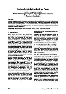
26 for species-specific estimates was seen with the dominant tree species. Features based on ALS intensity seemed to help in distinguishing the tree species. A lack of suitable neighbours caused errors especially in the highest end of the volume distribution. Using features selected for another study area produced higher RMSEs compared with those selected specifically for each area. The species-specific volume RMSEs rose more than those for total volume, except with deciduous species group in study area 1, which for some reason benefited from the use of features selected for study area 2. ALS-based features once again dominated in the reduced feature sets of V, which employed ALS and aerial photograph data in the estimation of forest biomasses (and volumes). The observations of Study IV above hold true for the ALS feature types selected into the final feature subsets. Here also, features based on ALS intensity were included in some of the final feature subsets. Nearly all aerial photograph features selected in study area 1 were various textural features based on grey level co-occurrence matrices. Spectral averages of grey values and various standard deviations were also included in the final feature subsets of study area 2. Fewer features were selected when the aim was to obtain the smallest possible RMSEs for total biomass or volume amounts, compared with the case where species-specific estimates were included in the objective function. Tree species inclusion in the objective function further increased the relative amount of aerial photograph-based features. When feature selection and estimation was based solely on the ALS-based features, slightly smaller RMSEs were obtained for total biomass and total volume in study area 1 than with the use of both feature types. There the GA was unable to eliminate unnecessary aerial photograph features. Combined feature sets produced smaller RMSEs in study area 2. The aerial photograph features were useful in both areas for species-specific estimation. Biases of total amounts were small in relation to the mean values. Species-specific biases were also small in study area 1, but the volume of deciduous species and biomasses of all species had some notable bias in study area 2. Figure 2 gives an idea of the mean volume RMSE levels obtained throughout Studies II to V. Note that the properties of study areas and numbers of field plots etc. vary from study to study. The observations arising from the figure are discussed in the next section.

5 DISCUSSION 5.1 Estimation and evaluation method The non-parametric k-NN estimation method was used throughout the studies. The benefit of this method is that it is simple and all desired inventory variables can be derived simultaneously. The method is non-parametric in the sense that no assumptions are made of the distributional characteristics of the auxiliary variables or the variables of interest. A commonly used statement of the method’s capability to preserve the covariances of the field variables seems to not hold true, at least for k > 1 (McRoberts 2009). Developing an analytical error estimation method for the entire target area, from pixel level to any area of interest, has been a challenge. Kim and Tomppo (2006), McRoberts et al. (2007) and Magnussen et al. (2009) have employed model-based methodology for this problem. The comparison of different image features is the point of view of the studies in this present dissertation, and the leave-one-out error estimates produced using the reference data set can be considered diagnostic enough.

40

60

80

STUDY V

ALS reduced, species-level volume criteria included, S2 ALS reduced, mean volume criterion only, S2 ALS + Aerial photo reduced, species-level volume criteria included, S2 ALS + Aerial photo reduced, species-level volume criteria included, S1 ALS reduced, species-level volume criteria included, S1 ALS + Aerial photo reduced, mean volume criterion only, S2 ALS + Aerial photo reduced, mean volume criterion only, S1 ALS reduced, mean volume criterion only, S1

20

STUDY IV

RMSE, % OF M E AN VOLUM E 0

STUDY III

ALS + Aerial photo reduced, large segments, S1 ALS + Aerial photo reduced, large segments, S2 ALS + Aerial photo reduced, small segments, S1 ALS + Aerial photo reduced, small segments, S2 ALS + Aerial photo reduced, plot-level, S2 ALS + Aerial photo reduced, plot-level, S1

STUDY II

TerraSAR-X all TerraSAR-X reduced ALS all ALS+TerraSAR-X all ALS reduced ALS +TerraSAR-X reduced

Landsat all Aerial photo all Landsat reduced Landsat reduced weighted Landsat all weighted Landsat + Aerial photo all Aerial photo all weighted Aerial photo reduced Landsat + Aerial photo all weighted Aerial photo reduced weighted Landsat + Aerial photo reduced Landsat + Aerial photo reduced weighted

27

Figure 2. Schematic comparison of relative mean volume RMSEs (% of the mean) obtained with different image data types and their combinations. Note that the properties of study areas and numbers of field plots etc. vary from study to study. The decrease of dimensionality of image features was based on GA.

28 Parameter selection used in the estimation has an impact on the k-NN-based results. The optimality of different image band combinations varied a bit according to the value of k (I). However, in other studies the value of k was fixed, because the comparison of image features from different sources was emphasised instead of method functionality. 5.2 Features originating from different sensors; their selection, combination and weighting As stated in subsection 1.2, the properties of remotely sensed data are a compromise between the spatial, spectral and radiometric resolution. A very good spatial resolution combined with mediocre spectral resolution present in aerial photography is slightly superior to good spectral resolution combined with mediocre spatial resolution present in multispectral satellite imagery (Study II; Tuominen and Poso 2001). Almost no differences were seen in studies comparing panchromatic imagery from SPOT satellite or aerial photographs (poor spectral resolution, good spatial resolution) with multispectral satellite imagery (Tokola et al. 1996; Hyyppä et al. 2000; Tuominen and Haakana 2005). The 3-D point cloud present in ALS data makes it strong compared with 2-D image material. ALS-based data was superior to TerraSAR-X radar data (III) and aerial photograph data (V). The suitability of separate image data types for forest variable estimation throughout the studies included in this dissertation can be summarised based on the order shown in Figure 2: ALS, TerraSAR-X, CIR aerial photographs, Landsat 7 ETM+. The RMSEs obtained using these data sources separately ranged from 23% to 77% of the mean volume of growing stock. A combination of features from different data sources mainly improved the accuracies (Studies II–V; Figure 2). Best results were obtained employing subsets of ALS and aerial photograph-based feature combinations, which in Studies IV–V gave mean volume RMSEs of 23–30%. These can be compared with 21–24% given by Packalén and Maltamo (2006; 2007), who also used combined subsets of both data types. Solely ALS-based features outperformed the combined subsets in Study V, in one study area, in the case of mean volume. The inclusion of TerraSAR-X radar data into ALS-based inventory also slightly decreased the RMSEs of mean characteristics, but the opposite occurred for species-specific volumes. A combination of aerial photograph and Landsat data always surpassed the use of a single data source for the forest variables included in II. A combination of Landsat-based features, acquired at different seasons or over a time span of several years, helped in discriminating the objects of interest (Study I, Franco-Lopez et al. 2001). Concerning the details of features selected from different image data types, it is interesting that even features based on ALS intensity were included in some of the feature subsets of Studies IV and V, despite the varying angle of incidence. However, those describing the vertical distribution of ALS observations clearly dominated. When aerial photograph features were combined with ALS or Landsat 7 ETM+ data, aerial photograph textural features were preferred over their basic grey values (Studies II, IV, V). Grey values from different wavelength regions were selected from each data source in a combination of aerial photograph and Landsat 7 ETM+ features (Study II). Lu (2005) found that textures were even more important than spectral responses in cases with complicated forest stand structure. A feature set with decreased dimensionality produced by automatic feature selection gave better results compared with the use of all available features (Studies II and III; Figure 2). The expansion of the feature space (large number of features) narrowed the set of field plots used as closest neighbours in tests carried out in Study II, concerning the curse of dimension-

29 ality. A simple genetic algorithm was used in II–V (also other methods in II). Although the randomness inherent in the applied genetic algorithm method results in somewhat random final feature subsets, logical differences occurred between features selected for different study areas. This observation also means that feature selection should be performed separately for each study area. However, there may usually be several good subsets within a large set of extracted image features. Based on the results obtained in Study II (and Packalén et al. 2012), it seems that feature selection can successfully be carried out in a multitude of ways. One phenomenon of the employed GA selection should be noted, though: the solely ALS-based feature subset outperformed the combined feature subset in one of the test cases, indicating that more flexibility should have been added to the process so as to allow for the eradication of all unfavourable features (aerial photograph features in this case). Optimal weights were searched for by adopting a downhill simplex method (I and II). Weighting was beneficial. Concerning the feature selection and weighting, overfitting of the models may occur, especially if the field dataset is small in relation to the number of features. The leaveone-out cross-validation helps to avoid this problem to a great extent: the target field plot is never itself present in the training data. However, feature selection and/or weighting emphasise features that minimise the RMSE of the forest variables of interest within the current field dataset. Above it was said that final feature sets differed logically between the study areas which is another aspect of this issue. The implications were studied in IV, where the features selected for one area were applied in the forest variable estimation of another area, and higher RMSE values were obtained. Species-specific volume errors were particularly affected. This is not surprising as the forest properties of these two areas greatly differed. In study area 1 the proportions of Scots pine, Norway spruce and deciduous species were relatively even whereas in study area 2 Norway spruce clearly dominated. In the case with one dominant tree species, features describing the vertical distribution of ALS height observations helped to discriminate between Norway spruce forests with various stocking, but were generally less useful for discriminating tree species groups in the other study area. The amount of mixed stands may also have varied, which would explain the failure of the features selected for study area 1 in the species-specific estimation of the Norway spruce dominated study area 2. This was, however, not explored further. The study area-specific training of models is one downside of data-driven selection of variables. However, as already stated in the Introduction, the complexity of relationships between ground truth and remotely sensed data gives justification for the use of automated methods. In the Methods it was mentioned that an earlier study showed the superiority of automatically selected features over those selected by researchers. Furthermore, the selection is not entirely data-driven: before initiating the feature selection process, the analyst has 1) selected the imagery and 2) selected the features to be extracted, both based on expert knowledge. There is also a third significant decision to be done by the analyst or the end user: which of the forest variables should be emphasized in the estimation process? One may e.g. put more weight on the estimation success of total stand volume than on tree species-specific volumes, and, as seen in the results of V, these choices affect the composition of the feature sets. The optimal parameter settings for k-NN also depend on the estimation targets. 5.3 Effects of illumination, topography and atmosphere No topographic, atmospheric or BRDF corrections were performed for the Landsat imagery in these studies. Topographic variation often has the greatest impact on the estimates in mountainous terrains, where topography-related variables may correlate more with image

30 values than the forest variables (Cohen and Spies 1992). The terrain was generally flat in the study areas included in this work. Atmospheric correction should be conducted when analysing single scenes if aerosols are heterogeneously distributed over the scene (Kaufman 1994). Here, the atmosphere was assumed uniform within single scenes. The dominant atmospheric effect is scattering for Landsat-type data, because bands have been designed to utilise the atmospheric transmission windows. The scattering effect is additive and the correction would be close to subtracting a constant in each spectral band, which has no meaning in the analysis of a single image (Song et al. 2001). Furthermore, it was possible to select cloud free imagery acquired in clear sky conditions. Concerning other image data types, only the central parts of the aerial photographs were used in II, to avoid part of the falloff and illumination problems. The imaging process in IV and V was digital, which removes or mitigates part of the distortions. All employed aerial photographs had been orthorectified using a DEM. The TerraSAR-X images were orthorectified to remove distortions caused by the side-looking imaging geometry (III). 5.4 Effects of forest area and field sample properties The effects of forest area characteristics could be seen in the results of two separate study areas used in IV and V. While the relative combined mean volume RMSEs of growing stock were approximately similar between the study areas (Figure 2), those for species-specific mean volumes differed greatly. The study areas were the same in both studies, but the plots in Study V with no tree biomass were removed. This had a negligible effect on the RMSEs of combined mean volume (27.8 to 27.5 and 29.6 to 28.5, in study areas 1 and 2, respectively). The effects on species-specific mean volumes were slightly larger. The high correlation between ALS data and structural stand variables has greatly improved the estimation results compared with those from medium resolution satellite imagery or aerial photographs. With k-NN the ALS-based features thus guide the nearest neighbour selection to those similar to the target stand also in reality, provided that these are present in the field data. The availability of similar field observations was tested by estimating the mean growing stock volumes as an average of five field observations with most similar volumes (II). The resulting RMSE was 7% of the mean volume. Even in this simple one-variable test an exact match would require more field plots. Scarcity of field observations in large volume classes seemed to increase the estimation error (IV). A lack of suitable neighbours was seen also in the results obtained with feature sets optimised for mean volume estimation only: the mean volume RMSEs decreased, but those of species-specific volumes rose, meaning that there were more eligible neighbours with similar volumes but the actual forest composition differed. Temesgen et al. (2003) and LeMay and Temesgen (2005) presented a further point: artificial new stand types may be created in an area-based approach with k-NN and similar methods, with tree species combinations that do not exist in the study area. This is of less importance in Nordic conditions, where the number of major tree species is small, and forests are regionally relatively homogeneous. Rare forest types may lack training data unless stratified sampling is applied when collecting field data. With stratified sampling, the efficiency of the inventory can furthermore be improved by allocating fewer field observations into strata that show little variation. Here, field data obtained using stratified sampling were available in Studies IV and V. Stratification can also be used in the estimation phase. Working within strata may improve the estimates by removing unsuitable training data observations before entering the process. For instance,

31 separate volume estimation for mineral soil forests and forests growing on peatland significantly decreased biases of both strata (Katila and Tomppo 2001). Data stratification into mineral soil and peatland forests was not possible due to the small number of field plots available, especially in the peatland strata (II to V). 5.5 Effects of spatial resolution and autocorrelation Estimation was carried out at the field inventory unit (or pixel/equidistant grid) level in the studies of this dissertation. As can be seen from the review given in Section 1.6, far better results have been reported for stand level, which is also the unit for silvicultural operations. In addition to inventory unit size, the shape may also be of importance. Employing combination of ALS and aerial photograph data, the idea of Study IV was to test the performance of automatically segmented substands, as it was thought that small, homogeneous segments around the field plot centre could also describe the field characteristics, possibly even better than a fixed-size grid element. However, these segments did not perform well, indicating that the segmentation failed to produce homogeneous segments. Part of the larger RMSEs was due to the complex segment forms, as borders were often generated in canopy gaps within the stands. Additional smoothing could have helped with this. Improved results were obtained using segments instead of field plots in studies with Landsat-type satellite imagery (Mäkelä and Pekkarinen 2001) and aerial photographs (Pekkarinen and Tuominen 2003). With satellite images, errors in image registration may be smoothed by using areas larger than one pixel. One factor to be taken into account is the possible discrepancy between field plot size and resolution of the remotely sensed data. In Study I the single subplots accounted only for 19% of the Landsat image pixel size. This undoubtedly had some effect on the estimation accuracy, however, when operating at the forest/non-forest level the effect should be smaller than in the case of stand volumes, forest cover classes etc. In Study II the field plot size (based on the maximum radius of the relascope sample plot) was 55% of the original Landsat pixel size, allowing a much better match. Other remote sensing data types contained several pixels or data points within the field plot areas, and gave the possibility to compute various statistical measures for each location, thus improving the separative capacity of the data. Concerning the spatial autocorrelation in I, preliminary trials using the leave-one-out cross-validation indicated a tendency for reference field plots to be chosen from the same field cluster as the target field plot, due to the close geographic distance. The analyses were thus also run by prohibiting neighbour selection from the same cluster. Field observations in other studies were assumed independent; the distances between field plots were larger than in I. 5.6 Other disturbance factors Estimation error includes a component caused by field measurement and variable modelling errors. Field plot location errors, image georeferencing errors, DTM construction errors with ALS data and differences between the imaging date and field data collection date cause mismatches between independent and dependent variables. These factors were not considered in this dissertation.

32 6 CONCLUSIONS This study focused on the potential that image features extracted from various remotely sensed data types served as independent variables for forest inventory purposes. Data sources included Landsat satellite images, aerial photographs, TerraSAR-X radar and ALS data. Combinatios of these data types were also employed. The potential was assessed based on forest variable estimation errors. In this study, large-area forest inventory was emphasized, but, the obtained methodology could be applied to forest inventories at both global and management levels. The effects of field sample properties (sampling design, location and measurement accuracy, models) were not considered in this dissertation. The estimation approach was area-based, which produces results for a uniform grid (or substand) instead of single-tree level estimation. The estimation method used was k-NN and automatic feature selection mainly based on a genetic algorithm process. According to the results, combining data sources with different, complementary properties typically improved the estimation accuracy of the studied forest variables. However, ALS-based features are quite powerful also when used separately. An automatically selected feature subset gives better estimates than a large number of features, due to noisy features and the ‘curse of dimensionality’. Forest area properties had an effect on the obtainable error levels, especially concerning the more detailed stand characteristics (species-level growing stock volumes), and also on the selected image feature subsets. Forests in this study were mainly located in Finland, meaning that they were under silvicultural management regimes, even-aged and typically had a clear stand structure. Finnish forests furthermore only have a few tree species. Generally, the more heterogeneous the forests are, the more indirect and irregular the relation between forest and spectral variables may be (Maselli and Chiesi 2006). The forest area types employed in this study are a good test bed for remote sensing-aided forest inventory methods – if the methods fail here, they will not work in more complex conditions either.

33 REFERENCES Aggarwal C.C., Hinneburg A., Keim D.A. (2001). On the surprising behavior of distance metrics in high dimensional space. In: Proceedings of the 8th International Conference on Database Theory (ICDT), London, UK, January 4–6. p. 420–434. Altman N.S. (1992). An introduction to kernel and nearest-neighbor nonparametric regression. The American Statistician 46(3): 175–185. Anttila P. (2002). Nonparametric estimation of stand volume using spectral and spatial features of aerial photographs and old inventory data. Canadian Journal of Forest Research 32(10): 1849–1857. http://dx.doi.org/10.1139/x02-108 Ardö J. (1992). Volume quantification of coniferous forest compartments using spectral radiance recorded by Landsat Thematic Mapper. International Journal of Remote Sensing 13(9): 1779–1786. http://dx.doi.org/10.1080/01431169208904227 Astrium GEO-Information Services. 2012. Discover the benefits of radar imaging. http:// www2.astrium-geo.com/files/pmedia/public/r15796_9_eij_radarimagery_finalarticle. pdf. [Cited 11 October 2014]. Balzter H., Baker J.R., Hallikainen M., Tomppo E. (2002). Retrieval of timber volume and snow water equivalent over a Finnish boreal forest from airborne polarimetric Synthetic Aperture Radar. International Journal of Remote Sensing 23(16): 3185– 3208. http://dx.doi.org/10.1080/01431160110076199 Beyer K.S., Goldstein J., Ramakrishnan R., Shaft U. (1999). When is ”Nearest Neighbor” meaningful? In: Proceedings of the 7th International Conference on Database Theory (ICDT), Jerusalem, Israel, January 10–12. p. 217–235. Boresjö Bronge L. (1999). Mapping boreal vegetation using Landsat-TM and topographic map data in a stratified approach. Canadian Journal of Remote Sensing 25: 460–474. http://dx.doi.org/10.1080/07038992.1999.10874745 Breidenbach J., Næsset E., Lien V., Gobakken T., Solberg S. (2010). Prediction of species specific forest inventory attributes using a nonparametric semi-individual tree crown approach based on fused airborne laser scanning and multispectral data. Remote Sensing of Environment 114: 911–924. http://dx.doi.org/10.1016/j.rse.2009.12.004 Campbell J.B. (2002). Introduction to remote sensing. Third edition. The Guilford Press, New York. 621 p.

34 Chang C. (2007). Overview. In: Chang C. (ed.) Hyperspectral data exploitation. Theory and applications. John Wiley & Sons, Inc., New Jersey. p. 1–16. http://dx.doi.org/10.1002/9780470124628.ch1 Chavez P.S., Berlin G.L., Sowers L.B. (1982). Statistical method for selecting Landsat MSS ratios. Journal of Applied Photogrammetric Engineering 8: 23–30 Cohen W.B., Spies T.A. (1992). Estimating structural attributes of douglas-fir/western hemlock forest stands from Landsat and Spot imagery. Remote Sensing of Environment 41: 1–17. http://dx.doi.org/10.1016/0034-4257(92)90056-P Congalton R.G. (1991). A review of assessing the accuracy of classifications of remotely sensed data. Remote Sensing of Environment 37: 35–46. http://dx.doi.org/10.1016/0034-4257(91)90048-B Cunia T. (1991). Main objectives and basic characteristics of national forest inventories. In: Köhl M., Pelz D. (eds.) Forest inventories in Europe with special reference to statistical methods. IUFRO Symposium, May 14–16, 1990, Birmensdorf, Switzerland. Swiss Federal Institute for Forest, Snow and Landscape Research, WSL/FMP, Birmensdorf, Switzerland. p. 27–33. Danaher T.J. (2002). An empirical BRDF correction for Landsat TM and ETM+ imagery. In: Proceedings of the 11th Australasian Remote Sensing and Photogrammetry Conference, 20–24 September 2002, Brisbane, Australia. p. 966–977. de Vries P.G. (1986). Sampling theory for forest inventory. A teach-yourself course. Springer-Verlag, Berlin. 399 p. http://dx.doi.org/10.1007/978-3-642-71581-5 Efron B., Tibshirani R.J. (1994). An introduction to the bootstrap. Chapman & Hall, New York. 456 p. European Space Agency. (2014). Synthetic Aperture Radar missions. http://www.esa. int/Our_Activities/Observing_the_Earth/Copernicus/SAR_missions. [Cited 9 March 2014]. Fazakas Z., Nilsson M., Olsson H. (1999). Regional forest biomass and wood volume estimation using satellite data and ancillary data. Agricultural and Forest Meteorology 98– 99: 417–425. http://dx.doi.org/10.1016/S0168-1923(99)00112-4 Federation of American Scientists. (2014). Electro-Optical Imaging Systems. https://www. fas.org/man/dod-101/navy/docs/es310/EO_image/EO_Image.htm. [Cited 9 March 2014]. Franco-Lopez H., Ek A.R., Bauer M.E. (2001). Estimation and mapping of forest density, volume and cover type using the k-nearest neighbors method. Remote Sensing of Environment 77: 251–274. http://dx.doi.org/10.1016/S0034-4257(01)00209-7

35 Franklin J. (1986). Thematic Mapper analysis of coniferous forest structure and composition. International Journal of Remote Sensing 7: 1287–1301. http://dx.doi.org/10.1080/01431168608948931 Franklin S.E., Hall R.J., Smith L., Gerylo G.R. (2003). Discrimination of conifer height, age, and crown closure classes using Landsat TM imagery in the Canadian Northwest Territories. International Journal of Remote Sensing 24(9): 1823–1834. http://dx.doi.org/10.1080/01431160210144589 Frazer G.W., Magnussen S., Wulder M.A., Niemann K.O. (2011). Simulated impact of sample plot size and co-registration error on the accuracy and uncertainty of LiDAR-derived estimates of forest stand biomass. Remote Sensing of Environment 115(2): 636–649. http://dx.doi.org/10.1016/j.rse.2010.10.008 Giri C., Zhu Z., Reed B. (2005). A comparative analysis of the Global Land Cover 2000 and MODIS land cover data sets. Remote Sensing of Environment 94: 123–132. http://dx.doi.org/10.1016/j.rse.2004.09.005 Goldberg D.E. (1989). Genetic algorithms in search, optimization, and machine learning. Addison-Wesley publishing company, Reading, Massachusetts. 412 p. Guyon I., Elisseeff A. (2003). An introduction to variable and feature selection. Journal of Machine Learning Research 3: 1157–1182. Haapanen R., Tuominen S. (2008). Data combination and feature selection for multi source forest inventory. PE&RS 4(7): 869–880. Haapanen R., Ek A.R., Bauer M.E., Finley A.O. (2004). Delineation of forest/nonforest land use classes using nearest neighbor methods. Remote Sensing of Environment 89: 265–271. http://dx.doi.org/10.1016/j.rse.2003.10.002 Haralick R. (1979). Statistical and structural approaches to texture. Proceedings of the IEEE 67(5): 786–804. http://dx.doi.org/10.1109/PROC.1979.11328 Haralick R., Shanmugan M.K., Dinstein I. (1973). Textural features for image classification. IEEE Transactions on Systems, Man and Cybernetics 3(6): 610–621. http://dx.doi.org/10.1109/TSMC.1973.4309314 Hinneburg A., Aggarwal C.C., Keim D.A. (2000). What is the nearest neighbor in high dimensional spaces? In: Proceedings of the 26th Very Large Data Bases (VLDB) Conference, September 10–14, Cairo, Egypt. p. 506–515. Holmgren P., Thuresson T., Holm S. (1997). Estimating forest characteristics in scanned aerial photographs with respect to requirements for economic forest management planning. Scandinavian Journal of Forest Research 12: 189–199. http://dx.doi.org/10.1080/02827589709355400

36 Holmström H., Nilsson M., Ståhl G. (2001). Simultaneous estimations of forest parameters using aerial photograph interpreted data and the k nearest neighbour method. Scandinavian Journal of Forest Research 16: 67–78. http://dx.doi.org/10.1080/028275801300004424 Holopainen M., Wang G. (1998). The calibration of digitized aerial photographs for forest stratification. International Journal of Remote Sensing 19(4): 677–696. http://dx.doi.org/10.1080/014311698215928 Holopainen M., Haapanen R., Tuominen S., Viitala R. (2008). Performance of airborne laser scanning- and aerial photograph-based statistical and textural features in forest variable estimation. In: Hill R., Rossette J., Suárez J. (eds.) Proceedings os Silvilaser 2008. p. 105–112. Holopainen M., Haapanen R., Karjalainen M., Vastaranta M., Hyyppä J., Yu X., Tuominen S., Hyyppä H. (2010). Comparing accuracy of airborne laser scanning and TerraSAR-X radar images in the estimation of plot-level forest variables. Remote Sensing 2010(2): 432–445. http://dx.doi.org/10.3390/rs2020432 Horler D.N.H., Ahern F.J. (1986). Forestry information content of Thematic Mapper data. International Journal of Remote Sensing 7(3): 405–428. http://dx.doi.org/10.1080/01431168608954695 Hudak A.T., Crookston N.L., Evans J.S., Hall D.E., Falkowski M.J. (2008). Nearest neighbor imputation of species-level, plot-scale forest structure attributes from LiDAR data. Remote Sensing of Environment 112(5): 2232–2245. Corrigendum: Remote Sensing of Environment 113(1): 289–290. http://dx.doi.org/10.1016/j.rse.2008.08.006 Hyvönen P. (2002). Kuvioittaisten puustotunnusten ja toimenpide-ehdotusten estimointi k-lähimmän naapurin menetelmällä Landsat TM -satelliittikuvan, vanhan inventointitiedon ja kuviotason tukiaineiston avulla. Metsätieteen aikakauskirja 3/2002: 363–379. Hyvönen P., Pekkarinen A., Tuominen S. (2005). Segment-level stand inventory for forest management. Scandinavian Journal of Forest Research 20: 75–84. http://dx.doi.org/10.1080/02827580510008220 Hyvönen P., Pekkarinen A., Tuominen S. (2007). Ilmakuvasegmentteihin perustuvan kaksivaiheisen otannan luotettavuus puustotunnusten ei-parametrisessa estimoinnissa. Metsätieteen aikakauskirja 1/2007: 39–53. Hyyppä J., Hyyppä H., Inkinen M., Engdahl M., Linko S., Zhu Y-H. (2000). Accuracy comparison of various remote sensing data sources in the retrieval of forest stand attributes. Forest Ecology and Management 128: 109–120. http://dx.doi.org/10.1016/S0378-1127(99)00278-9 Hyyppä J., Hyyppä H., Leckie D., Gougeon F., Yu X., Maltamo M. (2008). Review of methods of small-footprint airborne laser scanning for extracting forest inventory data in boreal

37 forests. International Journal of Remote Sensing 29(5): 1339–1366. http://dx.doi.org/10.1080/01431160701736489 Ilvessalo Y. (1950). On the correlation between the crown diameter and the stem of trees. Communicationes Instituti Forestalis Fenniae 28(2): 5–27. Jain R., Kasturi R., Schunck B.G. (1995). Machine vision. McGraw-Hill Inc., Singapore. 549 p. Jensen J.R. (1996). Introductory digital image processing: a remote sensing perspective. Second edition. Prentice Hall, New Jersey. 318 p. Jensen J.R. (2006). Remote sensing of the environment: an earth resource perspective. Prentice Hall, New Jersey. 608 p. Kalliovirta J., Tokola T. (2005). Functions for estimating stem diameter and tree age using tree height, crown width and existing stand database information. Silva Fennica 39(2): 227–248. Karjalainen M., Kankare V., Vastaranta M., Holopainen M., Hyyppä J. (2012). Prediction of plot-level forest variables using TerraSAR-X stereo SAR data. Remote Sensing of Environment 117: 338–347. http://dx.doi.org/10.1016/j.rse.2011.10.008 Karnieli A., Ben-Dor E., Bayarjargal Y., Lugasi R. (2004). Radiometric saturation of Landsat-7 ETM+ data over the Negev Desert (Israel): problems and solutions. International Journal of Applied Earth Observation and Geoinformation 5(2004): 219–237. http://dx.doi.org/10.1016/j.jag.2004.04.001 Katila M., Tomppo E. (2001). Selecting estimation parameters for the Finnish multisource National Forest Inventory. Remote Sensing of Environment 76: 16–32. http://dx.doi.org/10.1016/S0034-4257(00)00188-7 Katila M., Tomppo E. (2002). Stratification by ancillary data in multisource forest inventories employing k-nearest neighbour estimation. Canadian Journal of Forest Research 32: 1548–1561. http://dx.doi.org/10.1139/x02-047 Kaufman Y. (1994). The atmospheric effect on separability of field classes measured from satellite. Remote Sensing of Environment 18: 21–34. http://dx.doi.org/10.1016/0034-4257(85)90035-5 Kayitakire F., Giot P, Defourny P. (2002). Discrimination automatique de peuplements forestiers à partir d’orthophotos numériques couleur: un cas d’étude en Belgique. Canadian Journal of Remote Sensing 28: 629–640. http://dx.doi.org/10.5589/m02-058 Kilkki P., Päivinen R. (1987). Reference sample plots to combine field measurements and satellite data in forest inventory. Department of Forest Mensuration and Management, University of Helsinki. Research notes 19: 210–215.

38 Kim H-J., Tomppo E. (2006). Model-based prediction error uncertainty estimation for k-nn method. Remote Sensing of Environment 104: 257–263. http://dx.doi.org/10.1016/j.rse.2006.04.009 Korpela I. (2004). Individual tree measurements by means of digital aerial photogrammetry. Silva Fennica Monographs 3. 93 p. Latifi H., Nothdurft A., Koch B. (2010). Non-parametric prediction and mapping of standing timber volume and biomass in a temperate forest: application of multiple optical/ LiDAR-derived predictors. Forestry 83(4): 395–407. http://dx.doi.org/10.1093/forestry/cpq022 LeMay V., Temesgen H. (2005). Comparison of nearest neighbor methods for estimating basal area and stems per hectare using aerial auxiliary variables. Forest Science 51(2): 109–119. Lillesand T., Kiefer R. (1994). Remote sensing and image interpretation. John Wiley & Sons, Inc., New York. 750 p. Lu D. (2005). Aboveground biomass estimation using Landsat TM data in the Brazilian Amazon. International Journal of Remote Sensing 26(12): 2509−2525. http://dx.doi.org/10.1080/01431160500142145 Magnussen S., McRoberts R.E., Tomppo E.O. (2009). Model-based mean square error estimators for k-nearest neighbour predictions and applications using remotely sensed data for forest inventories. Remote Sensing of Environment 113: 476–448. http://dx.doi.org/10.1016/j.rse.2008.04.018 Maltamo M., Eerikäinen K., Pitkänen J., Hyyppä J., Vehmas M. (2004). Estimation of timber volume and stem density based on scanning laser altimetry and expected tree size distribution functions. Remote Sensing of Environment 90: 319–330. http://dx.doi.org/10.1016/j.rse.2004.01.006 Maltamo M., Malinen J., Packalén P., Suvanto A., Kangas J. (2006). Non-parametric estimation of stem volume using laser scanning, aerial photography and stand register data. Canadian Journal of Forest Research 36: 426–436. http://dx.doi.org/10.1139/x05-246 Maltamo M., Packalén P., Peuhkurinen J., Suvanto A., Pesonen A., Hyyppä J. (2007). Experiences and possibilities of ALS based forest inventory in Finland. In: Rönnholm P., Hyyppä H., Hyyppä J. (eds.) Proceedings of ISPRS Workshop on Laser Scanning 2007 and SilviLaser 2007. September 12–14, 2007, Espoo, Finland. p. 270−279. Marceau D.J., Gratton D.J., Fournier R.A., Fortin J-P. (1994). Remote sensing and the measurement of geographical entities in a forested environment. 2. The optimal spatial resolution. Remote Sensing of Environment 49(2): 105–117. http://dx.doi.org/10.1016/0034-4257(94)90047-7

39 Maselli F., Chiesi M. (2006). Evaluation of statistical methods to estimate forest volume in a Mediterranean region. IEEE Transactions on Geoscience and Remote Sensing 44 (8): 2239−2250. http://dx.doi.org/10.1109/TGRS.2006.872074 Mather P. (2004). Computer processing of remotely-sensed images: an introduction. Third edition. Wiley-Blackwell, Chichester. 442 p. McRoberts R.E. (2009). Diagnostic tools for nearest neighbors techniques when used with satellite imagery. Remote Sensing of Environment 113: 489–499. http://dx.doi.org/10.1016/j.rse.2008.06.015 McRoberts R.E., Nelson M.D., Wendt D.G. (2002). Stratified estimation of forest area using satellite imagery, inventory data, and the k-nearest neighbors technique. Remote Sensing of Environment 82: 457–468. http://dx.doi.org/10.1016/S0034-4257(02)00064-0 McRoberts R.E., Holden G.R., Nelson M.D., Liknes G.C., Gormanson D.D. (2006). Using satellite imagery as ancillary data for increasing the precision of estimates for the Forest Inventory and Analysis program of the USDA Forest Service. Canadian Journal of Forest Research 36: 2968–2980. McRoberts R.E., Tomppo E.O., Finley A.O., Heikkinen J. (2007). Estimating areal means and variances of forest attributes using the k-Nearest Neighbors technique and satellite imagery. Remote Sensing of Environment 111: 466–480. http://dx.doi.org/10.1016/j.rse.2007.04.002 Moeur M., Stage A.R. (1995). Most similar neighbor: an improved sampling inference procedure for natural resource planning. Forest Science 41: 337–359. Muinonen E., Tokola T. (1990). An application of remote sensing for communal forest inventory. In: Proceedings from SNS/IUFRO workshop: The usability of remote sensing for forest inventory and planning, 26–28 February 1990, Umeå, Sweden. Remote Sensing Laboratory, Swedish University of Agricultural Sciences, Report 4. p. 35–42. Muinonen E., Maltamo M., Hyppänen H., Vainikainen V. (2001). Forest stand characteristics estimation using a most similar neighbor approach and image spatial structure information. Remote Sensing of Environment 78: 223–228. http://dx.doi.org/10.1016/S0034-4257(01)00220-6 Mäkelä H., Pekkarinen A. (2001). Estimation of timber volume at the sample plot level by means of image segmentation and Landsat TM imagery. Remote Sensing of Environment 77: 66–75. http://dx.doi.org/10.1016/S0034-4257(01)00194-8 Mäkelä H., Pekkarinen A. (2004). Estimation of forest stand volume by Landsat TM imagery and stand-level field inventory data. Forest Ecology and Management 196(2–3): 245–255. http://dx.doi.org/10.1016/j.foreco.2004.02.049

40 Næsset E. (1997). Estimating timber volume of forest stands using airborne laser scanner data. Remote Sensing of Environment 51: 246–253. http://dx.doi.org/10.1016/S0034-4257(97)00041-2 Næsset E. (2004). Practical large-scale forest stand inventory using a small footprint airborne scanning laser. Scandinavian Journal of Forest Research 19: 164–179. http://dx.doi.org/10.1080/02827580410019544 Natural Resources Canada. (2013). Airborne versus spaceborne Radars. http://www.nrcan. gc.ca/earth-sciences/geomatics/satellite-imagery-air-photos/satellite-imagery-products/ educational-resources/9397. [Cited 11 October 2014]. Nelder J.A., Mead R. (1965). A simplex method for function minimization. Computer Journal 7(4): 308–313. http://dx.doi.org/10.1093/comjnl/7.4.308 Nilsson M. (1997). Estimation of forest variables using satellite image data and airborne lidar. Doctoral thesis. Acta Universitatis Agriculturae Sueciae 17. 31 p. Packalén P., Maltamo M. (2006). Predicting the plot volume by tree species using airborne laser scanning and aerial photographs. Forest Science 56: 611–622. Packalén P., Maltamo M. (2007). The k-MSN method in the prediction of species specific stand attributes using airborne laser scanning and aerial photographs. Remote Sensing of Environment 109: 328–341. http://dx.doi.org/10.1016/j.rse.2007.01.005 Packalén P., Maltamo M., Tokola T. (2008). Detailed assessment using remote sensing techniques. In: von Gadow K., Pukkala T. (eds.) Designing green landscapes. Managing Forest Ecosystems, vol. 15. Springer, Netherlands. p. 53–77. http://dx.doi.org/10.1007/978-1-4020-6759-4_3 Packalén P., Suvanto A., Maltamo M. (2009). A two stage method to estimate species specific growing stock by combining ALS data and aerial photographs of known orientation parameters. Photogrammetric Engineering and Remote Sensing 75(12): 1451–1460. http://dx.doi.org/10.14358/PERS.75.12.1451 Packalén P., Temesgen H., Maltamo M. (2012). Variable selection strategies for nearest neighbor imputation methods used in remote sensing based forest inventory. Canadian Journal of Remote Sensing 38(5): 557–569. http://dx.doi.org/10.5589/m12-046 Pekkarinen A. (2002). Image segment-based spectral features in the estimation of timber volume. Remote Sensing of Environment 82: 349–359 http://dx.doi.org/10.1016/S0034-4257(02)00052-4 Pekkarinen A., Tuominen S. (2003). Stratification of a forest area for multisource forest inventory by means of aerial photographs and image segmentation. In: Corona P., Köhl M.,

41 Marchetti M. (eds.) Advances in forest inventory for sustainable forest management and biodiversity monitoring. Forestry Sciences 76. Kluwer Academic Publishers. p. 111–123. Poso S., Wang G., Tuominen S. (1999). Weighting alternative estimates when using multi-source auxiliary data for forest inventory. Silva Fennica 33: 41–50. http://dx.doi.org/10.14214/sf.669 Press W.H., Teukolsky S.A., Vetterling W.T., Flannery B.P. (1999). Numerical recipes in C: the art of scientific computing. Second edition. Cambridge University Press, New York. 994 p. Sarvas R. (1938). Über die Bedeutung der Luftfotogrammetrie in unserer Waldwirtschaft. Silva Fennica 48: 1–45. http://dx.doi.org/10.14214/sf.a9072 Schowengerdt R.A. (2007). Remote sensing: models and methods for image processing. Third edition. Academic Press, New York. 515 p. Scott D.W., Sain S.R. (2005). Multi-dimensional density estimation. In: Rao C. R., Wegman E., Solka J. (eds.) Handbook of statistics 24: data mining and data visualization. Elsevier Publishing, New York. p. 229–262. Song C., Woodcock C.E., Seto K.C., Pax Lenney M., Macomber S.A. (2001). Classification and change detection using Landsat TM data: When and how to correct atmospheric effects? Remote Sensing of Environment 75: 230–244. http://dx.doi.org/10.1016/S0034-4257(00)00169-3 Spurr S.H. (1960). Photogrammetry and photo interpretation. With a section on applications to forestry. Second edition of Aerial photographs in forestry. The Ronald Press Company, New York. 472 p. St-Onge B.A., Cavayas F. (1997). Automated forest structure mapping from high resolution imagery based on directional semivariogram estimates. Remote Sensing of Environment 61: 82–95. http://dx.doi.org/10.1016/S0034-4257(96)00242-8 Stehman S.V. (1997). Selecting and interpreting measures of thematic classification accuracy. Remote Sensing of Environment 62: 77–89. http://dx.doi.org/10.1016/S0034-4257(97)00083-7 Stenberg P., Mõttus M., Rautiainen M. (2008). Modeling the spectral signature of forests: application of remote sensing models to coniferous canopies. In: Shunlin L. (ed.) Advances in land remote sensing. Springer, Netherlands. p. 147–171. http://dx.doi.org/10.1007/978-1-4020-6450-0_6 Suvanto A., Maltamo M., Packalén P., Kangas J. (2005). Kuviokohtaisten puustotunnusten ennustaminen laserkeilauksella. Metsätieteen aikakauskirja 4/2005: 413–428.

42 Temesgen H., LeMay V.M., Froese K.L., Marshall P.L. (2003). Imputing tree-lists from aerial attributes for complex stands of south-eastern British Columbia. Forest Ecology and Management 177(1–3): 277–285 http://dx.doi.org/10.1016/S0378-1127(02)00321-3 Thenkabail P.S., Enclona E.A., Ashton M.S., Legg C., Jean De Dieu M. (2004). Hyperion, IKONOS, ALI, and ETM+ sensors in the study of African rainforests. Remote Sensing of Environment 90: 23-43. http://dx.doi.org/10.1016/j.rse.2003.11.018 Tokola T. (2000). The influence of field sample data location on growing stock volume estimation in Landsat TM-based forest inventory in eastern Finland. Remote Sensing of Environment 74(3): 421–430. http://dx.doi.org/10.1016/S0034-4257(00)00135-8 Tokola T., Heikkilä J. (1997). Improving satellite image based forest inventory by using a priori site quality information. Silva Fennica 31(1): 67–78. http://dx.doi.org/10.14214/sf.a8511 Tokola T., Kilpeläinen P. (1999). The forest stand margin area in the interpretation of growing stock using Landsat TM imagery. Canadian Journal of Forest Research 29: 303–309. http://dx.doi.org/10.1139/x98-200 Tokola T., Pitkänen J., Partinen S., Muinonen E. (1996). Point accuracy of a non-parametric method in estimation of forest characteristics with different satellite materials. International Journal of Remote Sensing 17(12): 2333–2351. http://dx.doi.org/10.1080/01431169608948776 Tomppo E. (1991). Satellite image-based national forest inventory of Finland. International archives of photogrammetry and remote sensing 28: 419–424. Tomppo E. (1999). Forest inventory – a challenge for statistics. In: ISI 99. The 52nd Session of the International Statistical Institute, August 10–18, 1999, Helsinki, Finland. Proceedings, Tome LVIII, Book 1. Bulletin of the International Statistical Institute. p. 3–6. Tomppo E., Halme M. (2004). Using coarse scale forest variables as ancillary information and weighting of variables in k-NN estimation: a genetic algorithm approach. Remote Sensing of Environment 92: 1–20. http://dx.doi.org/10.1016/j.rse.2004.04.003 Tomppo E., Katila M., Moilanen J., Mäkelä H., Peräsaari J. (1998). Kunnittaiset metsävaratiedot 1990–94. Folia Forestalia 4B/1998: 619–839. Tomppo E., Olsson H., Ståhl G., Nilsson M., Hagner O., Katila M. (2008). Combining national forest inventory field plots and remote sensing data for forest databases. Remote Sensing of Environment 112: 1982–1999. http://dx.doi.org/10.1016/j.rse.2007.03.032

43 Trinder J. (2007). Characteristics of new generation of digital aerial cameras. http://www.geospatialworld.net/Paper/Technology/ArticleView.aspx?aid=2238 [Cited 9 March 2014]. Tuominen S. (2007). Estimation of local forest attributes, utilizing two-phase sampling and auxiliary data. Dissertationes Forestales 41. 46 p. + appendices. Tuominen S., Haakana M. (2005). Landsat TM imagery and high altitude aerial photographs in estimation of forest characteristics. Silva Fennica 39(4): 573–584. http://dx.doi.org/10.14214/sf.367 Tuominen S., Haapanen R. (2011). Comparison of grid-based and segment-based estimation of forest attributes using airborne laser scanning and digital aerial imagery. Remote Sensing 2011(3): 945–961. http://dx.doi.org/10.3390/rs3050945 Tuominen S., Haapanen R. (2013). Estimation of forest biomass by airborne laser scanning and digital aerial photographs. Silva Fennica 47(1), article id 902. 20 p. http://dx.doi.org/10.14214/sf.902 Tuominen S., Pekkarinen A. (2005). Performance of different spectral and textural aerial photograph features in multi-source forest inventory. Remote Sensing of Environment 94: 256–268. http://dx.doi.org/10.1016/j.rse.2004.10.001 Tuominen S., Poso S. (2001). Improving multi-source forest inventory by weighting auxiliary data sources. Silva Fennica 35: 203–214. http://dx.doi.org/10.14214/sf.596 Tuominen S., Fish S., Poso S. (2003). Combining remote sensing, data from earlier inventories and geostatistical interpolation in multi-source forest inventory. Canadian Journal of Forest Research 33(4): 624–634. http://dx.doi.org/10.1139/x02-199 Turner D.P., Cohen W.B., Kennedy R.E., Fassnacht K.S., Briggs J.M. (1999). Relationships between leaf area index and Landsat TM spectral vegetation indices across three temperate zone sites. Remote Sensing of Environment 70: 52–68. http://dx.doi.org/10.1016/S0034-4257(99)00057-7 Ulaby F.T., Moore R.K., Fung A.K. (1981). Microwave remote sensing. Active and passive. Volume 1. Microwave remote sensing fundamentals and radiometry. Artech House, London, UK. 456 p. USDA Forest Service. (2000). Forest inventory and analysis national core field guide, Volume 1: Field data collection procedures for phase 2 plots, version 1.4. USDA Forest Service, Internal report. On file at USDA Forest Service, Washington Office, Forest Inventory and Analysis, Washington, DC. van Coillie F.M.B, Lieven P.C., De Wulf R.R. (2005). GA-driven feature selection in object-based classification for forest mapping with IKONOS imagery in Flanders, Bel-

44 gium. In: Proceedings of ForestSat 2005, Borås May 3 – June 3. Rapport 8b. Swedish National Board of Forestry. p. 11–15. Vastaranta M., Wulder M.A., White J.C., Pekkarinen A., Tuominen S., Ginzler C., Kankare V., Holopainen M., Hyyppä J., Hyyppä H. (2013a). Airborne laser scanning and digital stereo imagery measures of forest structure: Comparative results and implications to forest mapping and inventory update. Canadian Journal of Remote Sensing 39(5): 382–395. http://dx.doi.org/10.5589/m13-046 Vastaranta M., Holopainen M., Karjalainen M., Kankare V., Hyyppä J., Kaasalainen S. (2013b). TerraSAR-X stereo SAR and airborne scanning LiDAR height metrics in imputation of forest above-ground biomass and stem volume. IEEE Transactions on Geoscience and Remote Sensing 52(2): 1197–1204. http://dx.doi.org/10.1109/TGRS.2013.2248370 Wall M. (1996). GAlib: A C++ Library of genetic algorithm components version 2.4 documentation, revision B. Massachusetts Institute of Technology. 101 p. Wang G., Waite, M-L., Poso, S. (1996). SMI user’s guide for forest inventory and monitoring. Department of Forest Resource Management Publications 16, University of Helsinki. 336 p. Woodcock C.E., Strahler A.H. (1987). The factor of scale in remote sensing. Remote Sensing of Environment 21: 311–332. http://dx.doi.org/10.1016/0034-4257(87)90015-0 Wulder M. (1998). Optical remote sensing techniques for the assessment of forest inventory and biophysical parameters. Progress in Physical Geography 22(4): 449–476. http://dx.doi.org/10.1177/030913339802200402 Wulder M., LeDrew E.S., Franklin S.E. (1998). Aerial image texture information in the estimation of Northern deciduous and mixed wood forest leaf area index (LAI). Remote Sensing of Environment 64: 64–76. http://dx.doi.org/10.1016/S0034-4257(97)00169-7 Yu X., Hyyppä J., Vastaranta M., Holopainen M., Viitala R. (2011). Predicting individual tree attributes from airborne laser point clouds based on random forest technique. ISPRS Journal of Photogrammetry and Remote Sensing 66: 28–37. http://dx.doi.org/10.1016/j.isprsjprs.2010.08.003