Explaining the Increased Polarization in the US Congress Daniel M. Butler∗ Stanford University Department of Political Science August 24, 2006
Abstract The increasing polarization between the two parties in the US Congress over the past several decades has been one of the great puzzles in American politics. In this paper I introduce a model in which the position chosen by candidates is determined by the tradeoff between alienating their base and persuading swing voters. I test the model by comparing its predictions with the actual DW-Nominate scores of the members of Congress both cross-sectionally and over time. The results provide strong support for the model and show how changes in the bases of the two parties have led to increasing congressional polarization.
1
Introduction From the perspective of politicians and political scientists there has been a drastic
change in the nature of US national politics over the past six decades. Over that period we have gone from a situation where centrist parties were concerned with persuading swing voters, to a situation in which parties take positions away from the center to mobilize their base. In response to the current congressional polarization, theoretical work has tried to develop models where candidates diverge in equilibrium. While much good work has come out of those efforts it has been insufficient. To explain the pattern observed during the post-war Congresses, we need a model that predicts both convergence and divergence behavior and explains when we should see each. I develop such a model here ∗
This is a condensed version of chapters 2 and 4 of my dissertation. I want to thank David Brady, Richard Butler, Morris Fiorina, Jay Goodliffe, Simon Jackman, and Matt Levendusky for feedback and suggestions on earlier drafts. Any remaining errors are my own.
1
by taking seriously what politicians say about how elections are conducted. Using data from a variety of sources, I test the model and show that it does a good job predicting candidate positioning and the pattern of polarization over the past several decades. Besides explaining candidate positioning and the current congressional polarization, the results in this paper have important implications for democratic theory. In the rest of this introduction, I motivate my model by reviewing the conventional wisdom on candidate positioning over the post-war period. Among the first generation of models trying to explain candidate positioning, the most influential was the Median Voter Theorem (Downs 1957; Black 1958). The theorem states that in a two candidate race, assuming that all voters turned out and voted for the candidate who took the position closest to their own ideal point, both candidates converge to the position of the median voter in order to maximize their probability of winning. Besides being simple and intuitive, the Median Voter Theorem seemed to do a good job explaining the politics that dominated the 1940s, 50s, and 60s. During those decades, the two parties took relatively centrist positions on most issues, most of the time. In fact, the lack of differences in the two parties led a committee of prominent political scientists to propose institutional reforms intended to give the parties incentives to take clear distinctive partisan stances (APSA 1950). As it turned out, the proposed institutional reforms were unnecessary because beginning in the 1970s the two political parties in Congress began to diverge from each other. Figures 1 and 2 plot the ideological differences between the two parties from the 93rd Congress (1973-1974) to the 108th Congress (2003-2004) for the House and Senate respectively. The top panel in both figures graphs the first dimension of the DW-Nominate scores1 of the two party medians over the past six decades. The difference between the two party medians for each Congress is given in the bottom panel of both figures. As the 1
DW-Nominate scores are computed by using the algorithm developed by Poole and Rosenthal which assigns each legislator an ideal point in a two dimensional space based upon their voting record in that Congress. The ideal points are assumed to be constant within a Congress but are allowed to change in a linear fashion over time. Since I am interested in the general ideological position of the legislators, I only use the score on the first dimension which is generally interpreted as the liberal-conservative position of the legislator.
2
figures show, the differences between the two parties has increased by about 35 percent in the House and 25 percent in the Senate ‘since the early 1970s. (Figure 1 about here) (Figure 2 about here) Accompanying the increased polarization in Congress, there has been a shift in the conventional wisdom on effective campaign strategies. The parties now emphasize the importance of mobilizing their base. For example, Matthew Dowd, one of George W. Bush’s senior advisors on his reelection campaign, said in 2003 that “there’s a realization, having looked at the past few elections, that the party that motivates their base - that makes their base emotional and turn out - has a much higher likelihood of success” (quoted in Nagourney 2003; cf. Fiorina 1999, 2-3; Miniter 2005; Millbank and Allen 2004). As these changes have occurred in politics, political science has revisited the question of candidate positioning. Empirically, work has shown the failure of the Median Voter Theorem’s convergence prediction in US elections (Ansolabhere, Snyder, and Stewart 2001; Lee, Moretti, and Butler 2004; Adams, Bishin, and Dow 2004). In response to that evidence, a large literature has developed suggesting ways to either modify or replace the Median Voter Theorem. The vastness of that literature is attested to by the fact that Fiorina (1999) and Grofman (2004) are full length articles dedicated to reviewing and summarizing that literature (see also Adams, Merrill, and Grofman 2005).2 As Fiorina 2
In his review of the literature, Fiorina (1999) identifies eight potential explanations that have been proposed to explain the observed candidate divergence: abstention (e.g. Hinich and Ordeshook 1969), policy-oriented candidates (e.g. Wittman 1977; Calvert 1985), citizen preferences (e.g. Aldrich 1983; Collie and Mason 1999), incumbency (e.g. Londregan and Romer 1993; Groseclose 1999), distributive politics (e.g. Kramer 1983), entry (e.g. Palfrey 1984), balancing (e.g. Fiorina 1988; Alesina and Rosenthal 1989), and parties (e.g. Austen-Smith 1984; Snyder 1994). Grofman’s (2004) review identifies another eleven potential explanations for candidate divergence in US elections: more than one round in the election (e.g. McGann 2002), more than one policy dimension, ambiguous policy positions of candidates (see Shepsle 1970; Aragones and Neeman 2000), votes based on perceived characteristics of each party’s support coalition (e.g. Owen and Grofman 1995), voters that look beyond the next election, turnout does not depend of voting costs versus expected benefits (e.g. Adams 2001; Adams and Merrill 2003), candidate policy location does not determine candidate support (e.g. Feld and Grofman 1991; Adams
3
(1999) points out, a major failing of the literature is that it has ignored the importance of turnout - especially variation in turnout out of one’s base - while political commentators have put increased importance on variation in participation as an explanation for candidate positioning (pp. 3, 28). I address this gap in the literature by incorporating into the model the conventional wisdom which suggests that a candidate’s base can to alienated when the candidate takes a position too far away from them (cf. Adams et al. 2006; Peres 2006). I also take seriously the importance of testing the model both cross-sectionally and over time. A model should not only explain why candidates diverge but also why they have polarized more over recent decades, and why that polarization has been asymmetric. As the patterns in Figures 1 and 2 show, congressional Republicans have moved further than congressional Democrats over the past three decades. In the rest of this paper I introduce a model of candidate positioning and then compare the predictions based on the model to the observed data. As I discuss below, there have been significant changes in the bases of the two parties over the past 30 years which explain the increasing polarization among candidates and its asymmetric nature.
2
Model of Candidate Positioning As noted in the introduction, I develop a model here to capture the conventional wis-
dom that mobilizing the party base can be an important candidate strategy. In creating that model, I incorporate two of three key characteristics of the unified theory of party competition from Adams, Merrill, and Grofman (2005). Specifically, I assume that partisan voters support their party’s candidate for non-policy reasons, but that those same partisans will abstain from voting if their candidate alienates them by moving too close to the center. The model developed here is most similar in terms of setup and intuition to parallel work being done by Adams et al. (2006), but extends their work by introducing 2000), probabilistic voting (e.g. Hinich 1977), voters inaccurately estimating the policy platforms of candidates (e.g. Granberg and Brent 1980), candidates looking beyond the next election (e.g. Budges 1994; Finegold and Swift 2001), and candidates who are not part of a unified team (e.g. Grofman, Koetzle, and Brunell 2000).
4
swing voters into the model. In Adams et al., voters are all either Democratic or Republican partisans. By including swing voters I am able to explicitly model the tradeoff that candidates face between mobilizing their base and persuading swing voters. In the rest of this section I discuss the intuition of the model and key comparative statics for the tests done in this paper; mathematical details of the model are provided in the appendix. In the model there are two candidates - a Republican and a Democrat - who play a one round game in which they simultaneously choose their ideological positions. In the game candidates are trying to maximize their margin of victory and are assumed to have complete information about how voters are distributed. Candidates maximize their margin of victory rather than simply their probability of winning because they want to win this election and put themselves in a better position for future elections. Having a higher margin of victory signals a candidate’s higher quality and helps to deter quality challengers in the future. In the model all voters belong to one of three groups - the Democratic base, the Republican base, or the swing voters. The swing voters are assumed to behave as classic Downsian voters (1957); all swing voters turn out to vote and vote for the candidate closest to them in ideological distance. Voters in the Democratic and Republican bases differ from swing voters in that party attachments matter a lot to them. One of the most important findings to come out of early survey research on voting is that party identification has a strong effect on vote choice (Campbell et al. 1960). To capture this dynamic in the model, the base voters are assumed to vote, if they vote, for the candidate of their party. While the candidates’ positions do not affect base voters’ preference over candidates, the positions do affect the turnout of the base. Specifically, the base voters who are far away from their candidate in the direction opposite of the median voter do not turn out.3 3
Note that this implies that while voters can abstain due to alienation, they do not abstain due to indifference. While previous research has shown that alienation does decrease turnout (Brody and Page 1973; Adams, Merril, and Dow 2005), this is still a strong assumption. I make it here because it simplifies the analysis without affecting the key intuition that candidates face a tradeoff between mobilizing their base and persuading swing voters (cf. Adams et al. 2006)
5
Finally, I assume that voters’ types are exogenous to the model. Significantly, this implies that the positions chosen by candidates do not affect which group a voter belongs to and that voters do not change types during an election. Since I am only modeling what occurs during an election, this assumption does not preclude the possibility of voters using cues from the political candidates to sort themselves into parties or change their ideology between elections (Levendusky 2006; for a related argument see McCarty, Poole, and Rosenthal 2006). In fact the two mechanisms could be working together. As candidates take more distinct positions, the voters sort into parties so that the bases move further apart for the next election, which in turn drives the candidates to take new positions during the next election that are further away from the median. The crucial point here is that during the few months covered by an election, voters are not significantly changing their ideology and party identification based on actions of the candidates (Campbell et al. 1960). Under these assumptions, candidates face a tradeoff between mobilizing their base and persuading swing voters. By moving towards the center, a candidate persuades more swing voters, but alienates more of her base who then do not turn out to vote. Symmetrically, if a candidate moves towards her base, those base voters turn out in higher numbers but it comes at the cost of losing ground among swing voters. The solution to the model is that candidates position themselves in such a way that if they moved they would lose more votes than they gained. Rather than doing a full analysis of the comparative statics of the model here, it is sufficient for the purposes of this paper to see how changes in the parameters of interest - the location and size of the candidates base and the size of the swing voters - affect candidate positions holding all else constant. These three relationships are given in figures 3-5.4 Figure 3 shows how the two candidates respond as the voters in their base change location. The kinks in the graph correspond to changes in which equilibrium the 4
In each of the figures, the parameters not being changed were held at the average values observed in the House districts for the election in 2000. The data was taken from the pooled cross-sections carried out as part of the Annenberg survey. See subsection 3.1 for full details.
6
candidates are in. For both candidates, as the base voters become more conservative (i.e. move to the right), the candidate’s position becomes more conservative. In other words, there is a positive relationship between the candidate’s position and the position of her base. (Figure 3 about here) (Figure 4 about here) Figures 4 and 5 show how candidates respond to changes in the size of their base and the swing voters respectively. Figure 4 shows that as a candidate’s base increases in size the candidate moves away from the median and toward the base. For Republican candidates this means that they become more conservative as their base gets larger, while Democrats become more liberal as their base gets larger. Figure 5 shows that both candidates move towards the center as the number of swing voters increases. Table 1 summarizes the predictions for the three variables for both candidates; in the next section I empirically test those predictions. A good sign about the relationships shown in Table 1 is that they fit our natural intuition. They also match the results from Adams, Merril, and Grofman (2005, 6061) on multi-candidate competition. These results are still significant because, to my knowledge, have not been previously derived for two-candidate competition. (Figure 5 about here) (Table 1 about here)
3
Testing the Model
3.1
Data from the 2000 Congressional Elections
To test the predictions of the model given in Table 1, I used data on members of the House and their constituents from the congressional elections in 2000 and the subsequent 7
107th Congress. As the dependent variable I used Poole and Rosenthal’s DW-Nominate scores for the members of the House in the 107th congress. The independent variables used in the analysis were created by using data from all cross-sectional samples in the 2000 National Annenberg Election Survey. One of the great advantages of the Annenberg Survey is the large number of respondents interviewed (an average of over 175 respondents per Congressional district). The only districts not represented are those from Hawaii and Alaska, where no surveys were conducted. To get the location (µ) and size (γ) of the three different types of voters in each district, I assigned respondents to be one of the three types of voters based on their initial response to the question about their self-identified party identification with independents being classified as swing voters. I then calculated the size of the groups by taking the proportion of each type in the district. To get the location of the different groups I flipped the scale of the ideology question asked in the Annenberg survey and used the mean ideology score for each group of voters as that group’s location. It was necessary to flip the scale (the scale now goes from 1=very liberal to 5=very conservative) so that it matched standard liberal-conservative scales, including the DW-Nominate scores, where increasing values indicate increasing levels of conservatism.
3.2
The Econometric Model
In this subsection I describe the econometric model used to test the predictions in Table 1. For the discussion below, I use the following definitions: yi = the DW-Nominate score for representative i µBi = the mean location of the base voters for representative i in i’s district γBi = the size of the base voters for representative i in i’s district γSi = the size of the swing voters in i’s district γOi = the size of the opposition’s base in i’s district An important feature of the data is that by construction we have that γBi +γSi +γOi = 1, which prevents us from including all three of these variables and a constant in the same regression because of perfect multicollinearity. While this means that we cannot
8
individually test the predictions concerning γBi and γSi , I will show below that we can still test them jointly. Ideally we would like to estimate the following equation:
yi = α + βµB µBi + βγB γBi + βγS γSi + βγO γOi + εi .
(1)
Because of the perfect multicollinearity we cannot estimate Eq. 1. Note, however, that if we substitute in for γSi (γSi = 1 − γBi − γOi ), we get the following equation:
yi = α + βµB µBi + βγB γBi + βγS (1 − γBi − γOi ) + βγO γOi + εi .
(2)
If we rearrange Eq. 2, we get the following equation which we can estimate:
yi = (α + βγS ) + βµB µBi + (βγB − βγS )γBi + (βγO − βγS )γOi + εi .
(3)
If we estimate Eq. 3, the coefficient on the size of the candidates own base (γBi ) is βγB − βγS which we can sign based on the predictions in Table 1. For the Democrats βγB − βγS should be negative (a negative number minus a positive number is a negative number) and positive for the Republicans (a positive number minus a negative number is a positive number). Table 2 gives a summary of the predictions for the regression based on Eq. 3. Note that no clear predictions are given for the coefficient on the size of the opposition’s base (γO ). (Table 2 about here)
3.3
Regression Results
I estimated the regression based on Eq. 3 for the Democrats and Republicans in the House separately and present the results in Table 3. Column 1 presents the results for the Democrats and column 2 the results for the Republicans. For both the Democrats and Republicans, changes in the location of the candidate’s own base has a positive effect on their DW-Nominate scores. In other words, as a candidate’s base gets more conservative, 9
the candidate takes a more conservative position. Not only do the coefficients have the correct sign, but they are statistically significant at conventional levels. (Table 3 about here) The coefficients on the the variable for the size of the candidate’s own base also take the predicted signs and are statistically significant at conventional levels. The coefficient is negative for the Democrat and positive for the Republican. The results on these two coefficients show that candidates respond not only to the location of the their own base, but also the sizes of their base and the swing voters. When one of those groups gets larger, the candidate moves towards it; increases in the size of the base leads candidates to move away from the center, while increases in the swing voters leads those candidates to move towards the center. The independent variables used in the regressions of Table 3 were measured assuming that all voters who identified with a party, whether weakly or strongly, were in that party’s base. A clear alternative is to assume that only strong party identifiers belong in the base. I reran the analysis using that definition of the base, and again found that all four coefficients had the predicted sign and were statistically significant at conventional levels. The results are available upon request.
3.4
Evaluating the Model’s Predictions of Candidate Positions
An even more direct way to evaluate the model is to compare the predictions of the model to the House members actual DW-Nominate scores (see Appendix for the mathematical details of the predictions). One issue about making predictions using the model is that in about 10 percent of the districts two equilibria were possible (but never more than two). The difference between the two equilibria was always that in one case both candidates were running closer to their base; in the other, one of the two candidates was running to the center in order to persuade swing voters. Because political practitioners have consistently emphasized the need to mobilize one’s base to win (see discussion in 10
Introduction), I assume that the equilibrium with both candidates mobilizing their base is focal.5 (Figure 6 about here) Figure 6 plots the House members’ actual DW-Nominate scores versus the predictions based on the model for the 107th Congress. The x-axis is a five point scale6 and the y-axis the typical scale used to calculate DW-Nominate scores. For the individual observations, the Republicans are represented by an R and the Democrats by a D. The patterns in Figure 6 show that the model is doing a good job predicting the positions of both parties.7 While the model seems to provide a good fit to the data, we would like to test whether the model provides information about candidate positioning beyond existing models. The model is only useful if it captures information not currently accounted for by previous work. For comparison, I choose three models that make point predictions of candidate positions and were close to some of the elements of the model developed here (we want to see if the model adds anything). Specifically, I compared my model to the Median Voter Theorem (MVT), the Primary Hypothesis, and the Two-stage Split Prediction. The MVT (Downs 1957; Black 1958) predicts that the candidates will converge to the position of the median voter. The prediction is operationalized by taking the ideological position of the median voter in the district. The Primary Hypothesis is that candidates represent the voters in the primary electorate (Fiorina, Abrams, and Pope 2004, ch. 8; see also Burden 2004). To operationalize the predictions of that hypothesis, I use the position of the median voter in the parties’ primary election.8 Finally, researchers have worked on 5
Assuming the other NE is focal does not change the conclusions reached in this subsection. 1=very liberal, 2=slightly liberal, 3=moderate, 4=slightly conservative, 5=very conservative 7 The strongest outlier is the Republican in the upper left portion of the graph. That observation is Paul Ryan, the representative of Wisconsin’s first congressional district. Because his district included a large number of independents who were on average slightly liberal, the model predicted that Representative Ryan should take a slightly liberal position to try to persuade them; his voting record suggests he did not. 8 In the Annenberg survey respondents were asked if they voted, or would vote (if the election had not taken place yet), in the presidential primary. If they answered affirmatively, they were asked to identify which party primary they participated in. For the Primary Hypothesis I take the median position of the voters who identified participating, or planning to participate, in the primary of the candidate’s party. 6
11
models where candidates must choose the optimal position to win in both the primary and general elections (Coleman 1971, 1972; Aranson and Ordeshook 1972; Wittman 1977, 1983, 1991; Owen and Grofman 1996; see also Gerber and Morton 1998). The basic idea behind these multistage models is that candidates will locate themselves between their primary and general constituencies to maximize their probability of winning both the nomination and the general election. I operationalize the Two-stage Split prediction by taking the midpoint between the median voters in the primary and general elections. (Table 4 about here) The bivariate correlation between the DW-Nominate Scores and the ideological positions predicted by the four models are given in Table 4. With the exception of the Median Voter Theorem all the models correlate highly with the representatives’ actual DW-Nominate scores, with the model developed here having the highest bivariate correlation. While the correlations are telling, they are insufficient to show that the model developed here is providing information not captured by the three competing models. To test whether my model is providing additional information about candidate positioning, we can run a regression where the representative’s DW-Nominate score is the dependent variable, and the predictions from the competing models are included as independent variables. Since OLS gives the best linear predictor of the dependent variable given the independent variables, if the other models are capturing all the information about candidate positioning, then the coefficient on the variable for the prediction of my model should be insignificant. + Here, as before, we have a case of perfect multicollinearity because MVT prediction 2 Primary prediction = Split prediction. As a result of the perfect multicollinearity, we 2 cannot estimate Equation 4, but we can estimate Equations 5-7 (see discussion in section 3.2):
12
DW-Nominatei = α + βM M My Model + βP Primary + βS Split + βM V T MVT + εi .
DW-Nominatei = α + βM M My Model + (βP +
(4)
βS βS )Primary + (βM V T + )MVT + εi . (5) 2 2
DW-Nominatei = α + βM M My Model + (βS + 2βP )Split + (βM V T − βP )MVT + εi . (6)
DW-Nominatei = α+βM M My Model+(βP −βM V T )Primary+(βS +2βM V T )Split+εi . (7) While we cannot use Equations 5-7 to test the validity of the Median Voter Theorem, Primary Hypothesis, and the Two-Stage Split Prediction, all three equations give an unbiased estimate of βM M , which allows us to test whether or not my model provides any information about candidate positioning which is not currently captured by the other three models. For completeness I report the results of all three models (Equations 5-7) in Table 5. The coefficient on the prediction from my model is substantively and statistically significant, showing that the model is providing information about candidate positioning that is not picked up by the other three models.9 (Table 5 about here) 9
Comparing the N in table 3 to those for Table 5 highlights that for 11 of the districts there was no Nash Equilibrium and hence no prediction. Since those 11 cases represent only 2.5 percent of all the 436 possible cases, it is unlikely that excluding them is driving the results. However to ensure the robustness of the results, I gave the 11 districts missing predictions for my model the values that were least favorable to my model and then reran the analysis in table 5. More specifically, I choose the values for those 11 observations that minimized the correlation between the prediction of my model and the DW-Nominate scores but still did not have the candidates playing strictly dominated strategies. While the results of the reanalysis were slightly weaker, not surprising given the added noise, they had the same substantive conclusion; the predictions of my model still provide information not captured by the three competing models. Full results available upon request.
13
4
Explaining Increased Congressional Polarization One of the major motivations for this research is to better understand why the parties
in the U.S. Congress have polarized over the past several decades. In this section I explore whether the model is predicting the over time trend in polarization. I first discuss how voters have changed over the past 30 years, and then compare the trends predicted by my model to the changes that are actually observed.
4.1
Changes in the Electorate over the Past Three Decades
In the previous sections I showed that candidates are responsive to the position and size of their base, and so move as their base does. Further, candidates respond to changes in the size of their own base in predictable ways. Specifically, as a candidate’s base gets larger, the candidate moves closer to it (and further away from the swing voters). These findings are significant given how the distribution of voters has changed over the past three decades. (Figure 7 about here) Figure 7 shows the distribution the three types of voters in the US in 1972 (in the top panel) and 2004 (in the bottom panel). The data come from the American National Election Study’s surveys in the respective years and represent the US population as a whole. Respondents were assigned to be one of the three types of voters based upon their initial response to the question about their self-identified party identification.10 Between 1972 and 2004, there has been almost no change among the swing (or independent) voters; in both years their modal position is 4 and their mean position 4.02. Further, in both years they represent roughly 35 percent of the electorate. In contrast to the swing voters, the bases of the two parties have changed significantly. The mean liberal-conservative position for Republicans has gone from 4.71 to 5.25. The 10
Swing voters included independents as well as any other unaffiliated voters (but not voters identifying with smaller third parties).
14
Republicans have also increased in number, going from roughly 27 percent of the electorate in 1972 to nearly 35 percent in 2004. For Democrats the mean has shifted from 3.84 in 1972 to 3.28 in 2004. At the same time, the number of Democratic identifiers has decreased from 38 percent of the electorate in 1972 to 30 percent in 2004. In sum, the Republicans have become larger and moved to the right, while the Democrats have become smaller and moved to the left. For the Republican candidates these changes should both work to induce them to move right and to take a more conservative position. Because these changes reinforce each other, the model yields a clear prediction of increasing conservatism among Republican candidates. For Democrats on the other hand, the two changes in the base are opposing forces. The movement of the base to the left should give the Democratic candidates incentives to move left. However, the decreasing size of the base works in the opposite direction giving Democratic candidates more incentives to try to appeal to swing voters by moving right. Since these two changes are working in opposite directions, it is unclear what the optimal Democratic response to the changes in the composition of the Democratic base should be. This information already provides some indication that the model may be capturing the important dynamics of candidate positioning. As discussed in the introduction, the increased distance between the two parties over the past three decades has been asymmetric in character, being driven disproportionately by movement of the Republicans in a conservative direction (see Figures 1 and 2). Given how the distribution of voters has changed over the past three decades (Figure 7), the movement on the part of the Republicans and the relative lack of change among the Democrats is in accordance with the model developed here.
4.2
Creating a Mock Senate Based on the Model Predictions
To investigate whether the model predicts the changes we observe in the position of the two parties in Congress, I used survey data collected over the past three decades to create 15
a mock Senate populated with legislators whose ideological positions were predicted by the model developed in this paper. I do not test the other models because voters were asked about participation in primary elections in only about one third of the NES surveys over the time period making it so there are not enough observations for the empirical tests done here. To get the Senators’ predicted positions based I used data from the National Election Studies main surveys from 1972-2002. I begin in 1972, because that is the first year the NES asked respondents to place themselves on a seven point liberal-conservative scale, which is necessary information for making predictions about candidate positioning using the model. The surveys from 2004 were excluded because the corresponding DWNominate scores are not yet available since the 109th Congress is still in session. Because I use the data to estimate three different distributions in the state, I only used the states where there were at least 20 respondents placing themselves on the seven point liberalconservative scale. Using this cut-off rule meant that over the 16 surveys available I used an average of 22.5 states for each Congress when creating the mock Senate.11 For each of the states with enough available respondents, I used the estimates of the voter distributions to get predictions based on the model of what positions the Democratic and Republican candidates should take. I then populated the mock Senate for the Congress corresponding to that survey year, with two observations per state whose party identification corresponded to the party that controlled the two Senate seats in that state, giving each observation the position predicted by the model for that party in that state. So, for example, the Iowa Senate delegation to the 102nd Congress included a Republican, Chuck Grassley, and a Democrat, Tom Harkin. Using the survey data from Iowa in 1990 (the election year corresponding to the 102nd Congress), the model predicted that the Democrat should take a position on the seven point scale of 2.77 while the Republican candidate should position himself at 5.83. In creating the mock Senate for the 100th Congress, I put in a Democrat taking the position at 2.77 and a Republican 11
I also checked if using a higher cut-off point would affect the results. It did not.
16
at the position of 5.83, to represent Tom Harkin and Chuck Grassley respectively. I then created a complementary Senate based on actual DW-Nominate scores from the Senators for that Congress. For the Iowa Senate delegation to the 102nd Congress, this meant putting in Tom Harkin’s score of -0.524 for the Democrats and Chuck Grassley’s score of 0.314 for the Republicans. I created this complementary Senate, so I could directly compare the predictions made by my model to the actual voting scores of the same Senators. Using the DW-Nominate scores for the full Senate is inappropriate because I do not have predicted positions for all the different Senators due to lack of survey respondents in smaller states.
4.3
Testing the Model’s Predictions Over Time
I first investigate whether my model predicts the over time trend in polarization in the Senate as measured by the difference between the two party medians. To carry out that test, I first scaled the polarization trend line for the Mock Senate based on the predictions of my model so that it had the same mean as the polarization trend line for the Real Senate. Figure 8 displays the resulting trend lines and shows that the model developed here seems to be doing a good job predicting the over time trend. (Figure 8 about here) More formally, we can test whether the two lines are indistinguishable by first defining the following variables: yi = the distance between the party medians (predicted or actual) T imei = a variable ranging from 0 (93rd Congress) to 15 (108th Congress) M ocki = 1 if the observation is a prediction from my model and 0 otherwise We can then estimate Equation 8 and test the joint hypothesis that βM = βM T = 0. In words, I am simply testing whether the two lines have the same intercept and slope. To do that test, I estimated Equation 8 and performed the associated test and present the results in Table 6. As the results show, there is no evidence that the trend lines are 17
different; we cannot reject that the two lines have the same intercept and slope.
yi = α + βM M ocki + βT T imei + βM T M ock ∗ T imei + εi .
(8)
(Table 6 about here) As discussed in the introduction, the divergence in DW-Nominate scores over time has been asymmetric with Republicans moving more than their Democratic counterparts over the past 30 years. To see if the predictions from the model being used in the mock Senate captured that dynamic, I graphed the trends in party medians over time for both the Mock and Real Senates in Figure 9. In the Real Senate, the Republicans have moved 0.224 points in the conservative direction (from 0.133 to 0.357), while the Democrats have only moved 0.066 points in the liberal direction (-0.387 to -0.453). So the Republican movement right accounts for 77% of the increased divergence observed between the two parties in Congress over the past 30 years.12 The predictions of the model given in the Mock Senate do a good job capturing that dynamic. The Mock Senate predictions have the Republican median moving 0.938 points in the conservative direction (4.955 to 5.893) and the Democrats only 0.525 in the liberal direction (3.428 to 2.903). Significantly that means that the predictions of the Mock Senate predicted that the Republicans are responsible for 64% of the increased divergence.13 These results, combined with those from earlier sections, suggest that the changes in the bases of the two parties have driven the observed pattern of congressional polarization. (Figure 9 about here) 0.224 (0.224+0.066) 0.938 13 (0.938+0.525) 12
= 0.77 = 0.64
18
5
Discussion Because of its simple intuition, the Median Voter Theorem is still the dominant theo-
retical paradigm for understanding candidate behavior; however, much research has been done showing its empirical weaknesses in explaining observed candidate behavior. The results here show how we can extend and modify that model to better explain real politics. Developing better models will improve the research on such issues as candidate positioning, policy formation, and representation. In addition, the model and empirical evidence in this paper provide an explanation for why we have observed a divergence of the two parties in Congress over the past three decades. Voters in the parties’ bases are now taking more extreme ideological positions than before, causing the candidates to move away from the center. The Republican members of Congress have moved more over the past 30 years because their base has become larger and moved right while the Democratic base has become smaller and moved left. The increased size has made Republicans even more responsive to the conservative positions of their base. Besides explaining why candidates have diverged, the findings of this research imply that candidates in U.S. congressional elections still respond to the preferences of their constituencies. This contradicts the claims made that the Republicans have become more conservative in spite of the preferences of voters (e.g. Frank 2004; Hacker and Pierson 2005). While parties may not be responding to the position of the median voter, they are still responding to the preferences of their constituencies. The findings of this research may also help explain the strong empirical relationships that McCarty, Poole, and Rosenthal (2006) uncover. While McCarty, Poole, and Rosenthal show that there is a positive relationship between polarization in Congress and the levels of income inequality and immigration, they do not provide a satisfactory explanation for why. In light of the findings here, the increasing immigration and income inequality could explain the changes in the sizes and ideological preferences of the two
19
parties’ bases, which in turn explain the increased polarization between the two parties. First, the increase in income inequality could explain the observed polarization of the preferences of the voters in the parties’ bases over the past thirty years. As inequality increases, the voters in the party representing wealthier interests (the Republicans) should desire less redistribution because they have more to lose, while the voters in the base of the party representing those with lower incomes (the Democrats) should desire more redistribution as inequality increases because they have more to gain. The observed shifts to the right and left of the Republican and Democrat identifiers respectively fit that description (see Figure 7). Second, the higher immigration rates might explain the increased number of Republican identifiers among voters. As McCarty, Poole, and Rosenthal show the non-citizens who have come to the US during the recent waves of immigration have been poorer than the average American citizen, making the median voter wealthier relative to the median worker (ch. 4). As the median voter becomes wealthier relative to the median worker, the number of voters against redistribution should increase which in turn should increase the number of Republican identifiers. Future research should be done to see if income inequality and immigration have worked to increase polarization by changing the sizes and preferences of the two parties’ bases as described here. The results also suggest several other questions for future theoretical and empirical research. Future theoretical work could try to capture the effect of incumbency by seeing if the results of the model change when one candidate gets to move first. Work could also be done to see if the results change when the bases in the parties differ in how easily they are alienated. The model presented here assumes that the parameter a, the alienation distance, is symmetric for both parties. By relaxing that assumption, research could investigate how candidates react when the voters in their base are more fickle than their opposition’s base. Empirically, future research should be done to see whether compulsory voting makes candidates and campaigns more moderate. In the model, the reason that candidates 20
diverge from the median is to mobilize base voters. In a system with compulsory voting the increased cost to abstention leads more voters to turn out, making mobilization of base voters less of a priority for candidate and thereby causing candidates to move towards the center to capture swing voters. As Jackman (2004) points out, the effect of compulsory voting on campaigns is almost completely unexplored. Given that compulsory voting is one of the major electoral institutions that differs across the developed democracies, exploring its effect on candidate behavior is an important area for future research.
References Adams, James. 2001. Party Competition and Responsible Party Government: A Theory of Spatial Competition Based upon Insights from Behavioral Voting Research. Ann Arbor: University of Michigan Press. Adams, James, Benjamin Bishin, and Jay Dow. 2004. “Representation in Congressional Campaigns: Evidence for Directional/Discounting Motivations in United States Senate Elections.” Journal of Politics 66(2): 348-373. Adams, James, Samuel Merrill, III, and Bernard Grofman. 2005. A Unified Theory of Party Competition: A Cross-National Analysis Integrating Spatial and Behavioral Factors. Cambridge: Cambridge University Press. Adams, James, Thomas L. Brunell, Bernard Grofman, and Samuel Merrill, III. 2006. “Move to the Center or Mobilize the Base? Effects of Political Competition, Vote Turnout, and Partisan Loyalties on the Ideological Divergence of Vote-Maximizing Candidates.” Typescript. University of California, Davis. Adams, James, Jay Dow, and Samuel Merrill. Forthcoming. “The Political Consequences of Alienation-Based and Indifference-Based Vote Abstention: Applications to Presidential Elections.” Political Behavior. Adams, James, and Samuel Merrill. 2003. “Voter Turnout and Candidate Strategies in American Elections.” Journal of Politics 65(1): 161-189. Aldrich, John. 1983. “A Downsian Spatial Model with Party Activism.” American Political Science Review 77: 974-990. Alesina, Alberto, and Howard Rosenthal. 1989. “Partisan Cycles in Congressional Elections and the Macroeconomy.” American Political Science Review 83: 373-98.
21
Ansolabhere, Stephen, James M. Snyder, Jr., and Charles Stewart, III. 2001. “Candidate Positioning in U.S. House Elections.” American Journal of Political Science 45 (1): 136-159. APSA Committee on Political Parties. 1950. “Toward a More Responsible Two-Party System” American Political Science Review 44 (3, part 2, supplement): 1-96. Aragones, Enriqueta, and Zvika Neeman. 2000. “Strategic Ambiguity in Electoral Competition.” Journal of Theoretical Politics 12(2): 183-204. Aranson, Peter H., and Peter C. Ordeshook. 1972. “Spatial Strategies for Sequential Elections.” in R. Niemi and H. Weisberg, eds. Probability Models of Collective Decision Making. Columbus, Ohio: Charles E. Merrill. Austen-Smith, David. 1984. “Two-Party Competitions with Many Constituencies.” Mathematical Social Sciences 7: 177-198. Berelson, Bernard R., Paul F. Lazarfeld, and William N. McPhee. 1954. Voting: A Study of Opinion Formation in a Presidential Campaign. Chicago: University of Chicago Press. Black, Duncan. 1958. The Theory of Committees and Elections. Cambridge: Cambridge University Press. Brody, Richard, and Benjamin Page. 1973. “Indifference, Alienation, and Rational Decisions: The Effects of Candidate Evaluation on Turnout and Vote.” Public Choice 15: 1-17. Budge, Ian. 1994. “A New Spatial Theory of Party Competitions: Uncertainty, Ideology, and Policy Equilibria Viewed Comparatively and Temporally.” British Journal of Political Science 24: 443-467. Burden, Barry C. 2004. “Candidate Positioning in US Congressional Elections.” British Journal of Political Science 34: 211-227. Calvert, Randall. 1985. “Robustness of the Multidimensional Voting Model: Candidate Motivations, Uncertainty, and Convergence.” American Journal of Political Science 29: 69-95. Campbell, Angus, Philip E. Converse, Warren E. Miller, and Donald E. Stokes. 1960. The American Voters. Chicago: University of Chicago Press. Collie, Melissa, and John Mason. 1999. “The Electoral Connection Between Party and Constituency Reconsidered.” In Continuity and Change in House Elections. Edited by David Brady, John Cogan, and Morris Fiorina. Stanford, CA: Stanford University Press. Coleman, James S. 1971. “Internal Processes Governing Party Positions in Elections.” 22
Public Choice 11: 35-60. Coleman, James S. 1972. “The Positions of Political Parties in Elections.” in R. Niemi and H. Weisberg, eds. Probability Models of Collective Decision Making. Columbus, Ohio: Charles E. Merrill. Downs, Anthony. 1957. An Economic Theory of Democracy. New York: Harper and Row. Finegold, Kenneth, and Elaine K. Swift. 2001. “What Works? Competitive Strategies of Parties out of Power.” British Journal of Political Science 31: 95-120. Fiorina, Morris. 1988. “The Reagan Years: Turning to the Right or Groping Towards the Middle?” In The Resurgence of Conservatism in Britain, Canada and the United States. Edited by Barry Cooper and Allan Kornberg. Durham, N.C.: Duke University Press: 430-460. Fiorina, Morris P. 1999. “Whatever Happened to the Median Voter?” Presented at the MIT Conference on Parties and Congress, Cambridge, MA, October 2, 1999. Fiorina, Morris P., Samuel J. Abrams, and Jeremy C. Pope. 2004. Culture War? The Myth of a Polarized America. New York: Pearson Longman. Franks, Thomas. 2004. What’s the Matter with Kansas? How Conservatives Won the Heart of America. New York: Metropolitan Books. Gerber, Elizabeth, and Rebecca B. Morton. 1998. “Primary Election Systems and Representation.” Journal of Law, Economics, and Organization 11(2): 304-324. Granberg, Donald, and Edward Brent. 1980. “Perceptions and Issue Positions of Presidential Candidates.” American Scientist 68: 617-685. Grofman, Bernard. 2004. “Downs and Two-Party Convergence.” Annual Review of Politcal Science 7: 25-46. Grofman, Bernard, William Koetzle, and Thomas Brunell. 2000. “A New Look at Split Ticket Voting for House and President: The Comparative Mid-points Model.” Journal of Politics 62(1): 34-50. Groseclose, Tim. 2001. “A Model of Candidate Location when one Candidate has a Valence Advantage.” American Journal of Political Science 45 (4): 862-886. Hacker, Jacob S., and Paul Pierson. 2005. Off Center: The Republican Revolution & the Erosion of American Democracy. New Haven: Yale University Press. Hinich, Melvin, and Peter Ordeshook. 1969. “Abstention and Equilibrium in the Elec23
toral Process.” Public Choice 7: 81-106. Hinich, Melvin. 1977. “The Median Voter is an Artifact.” Journal of Economic Theory 16: 208-219. Jackman, Simon. 2004. “Compulsory Voting.” in Elseviers International Encyclopedia of the Social and Behavioral Sciences. Kramer, Gerald. 1983. “Electoral Politics in the Zero-Sum Society.” Social Science Working Paper 472. Pasadena, CA: Caltech. Lacy, Dean, and Barry Burden. 1999. “The Vote-Stealing and Turnout Effects of Ross Perot in the 1992 United States Presidential Election.” American Journal of Political Science 43: 233-255. Lee, David S., Enrico Moretti, and Matthew J. Butler. 2004. “Do Voters Affect or Elect Policies? Evidence from the U.S. House.” Quarterly Journal of Economics 119 (3): 807859. Levendusky, Matthew S. 2006. Sorting, not Polarization: The Dynamics of Electoral Change, 1972-2004. Dissertation. Stanford University, Stanford, CA. Londregan, John, and Thomas Romer. 1993. “Polarization, Incumbency, and the Personal Vote.” In Political Economy: Institutions, Competition, and Representation. Edited by William Barnett, Melvin Hinich, and Norman Schofield. New York: Cambridge: 355-377. McCarty, Nolan, Keith Poole, and Howard Rosenthal. 2006. Polarized America: The Dance of Ideology and Unequal Riches. Cambridge: MIT Press. McGann, A.J. 2002. “The Advantages of Ideological Cohesion: A Model of Constituency Representation and Electoral Competition in Multi-party Democracies.” Journal of Theoretical Politics 14(1): 37-70. Millbank, Dana, and Mike Allen. 2004. “Bush Fortifies Conservative Base: Campaign Seeks Solid Support Before Wooing Swing Voters.” Washington Post, July 15. Miniter, Branden. 2005. “The McCain Myth: The Moderation that Makes Him a Senate Powerhouse Will Keep Him Out of the White House.” Wall Street Journal, May 31. Nagourney, Adam. 2003. “Political Parties Shift Emphases to Core Voters.” New York Times, August 30. Owen, Guillermo, and Bernard Grofman. 1996. Two-stage Electoral Competition in Two-party Contests: Persistent Divergence of Party Positions with and without Expressive Voting. Presented at Conf. Strategy and Politics, Center for the Study of Collective 24
Choice, University Maryland, College Park, MD, April 12. Palfrey, Thomas. 1984. “Spatial Equilibrium with Entry.” Review of Economic Studies 51: 139-156. Peress, Michael. 2005. “Securing the Base: Electoral Competition under Variable Turnout.” Typescript. Carnegie Mellon University. Shepsle, Kenneth A. 1970. “Uncertainty and Electoral Competition: The Search for Equilibrium.” American Political Science Review 23: 27-59. Snyder, James. 1994. “Safe Seats, Marginal Seats, and Party Platforms: The Logic of Platform Differentiation.” Economics and Politics 6: 201-214. Wittman, Donald. 1977. “Candidates with Policy Preferences: A Dynamic Model.” Journal of Economic Theory 14: 180-189. Wittman, Donald A. 1983. “Candidate Motivations: A Synthesis of Alternatives.” American Political Science Review 77: 142-157. Wittman, Donald A. 1991. “Spatial Strategies When Candidates Have Policy Preferences.” in J. Enelow and M. Hinich, eds. Advances in the Spatial Theory of Voting. Cambridge: Cambridge University Press, pp. 66-98.
Appendix For the discussion here about the model, let the subscripts S, R, and D, represent the swing voters, the Republicans (candidates and voters), and the Democrats (candidates and voters) respectively. In the model the candidates play a one round game where both players simultaneously choose an ideological position to take, YR and YD , while trying to maximize their margin of victory. I assume that all voters belong to one of three groups - the Democratic base, the Republican base, or the swing voters. I let γi represent the proportion of the population in the district that belongs to group i; by construction then we have that γD + γS + γR = 1. I assume that the ideal points for each group i are distributed with mean µi and spread σi and that µD < µS < µR . The swing voters are assumed to behave as classic Downsian voters (1957); all the swing voters turn out to vote and vote for the candidate closest in distance to them. 25
Because we are interested in how this affects the vote total for the two candidates, we can multiply the size of the swing voters (γS ) by the percentage of them voting for each candidate. Equations 9 and 10 give the resulting total for the Democratic and Republican candidates respectively (Fi represents the cdf of the distribution for voter group i).
Democratic Vote from Swing Voters = γS ∗ [FS (
YD YR + )]. 2 2
Republican Vote from Swing Voters = γS ∗ [1 − FS (
YD YR + )]. 2 2
(9)
(10)
The voters in the Democratic and Republican bases differ from swing voters in that party attachments matter a lot to them. One of the most important findings to come out of early survey research on voting is that party identification has a strong effect on vote choice (Berelson, Lazarfeld, McPhee 1954; Campbell et al. 1960). To capture this dynamic in the model, the base voters are assumed to vote, if they vote, for the candidate of their party. While the candidates’ positions do not affect base voters’ preference over candidates, the positions do affect the turn out decision of the base. Specifically, the model assumes that all the base voters who are further than a,14 which I refer to as the alienation distance, away from the candidate in the direction opposite of the median voter do not turn out.15 For the Democrats, this means that all the base voters who have a position further left than the point YD − a do not turn out to vote. For Republicans, it is all the voters in their base who have a position further right than the point YR + a that do not vote. Equation 11 gives the vote share that the Democratic candidate gets from her base as a function of her position and the mean and spread of the base voters. Equation 12 provides the same information for the Republican candidate. 14
Alternatively, one could allow this ‘distance’ to differ across individuals (see Lacy and Burden 1999). Note that this implies that while voters can abstain due to alienation, they do not abstain due to indifference. While previous research has shown that alienation does decrease turnout (Brody and Page 1973; Adams, Merril, and Dow 2005), this is still a strong assumption. I make it here because it simplifies the analysis without affecting the key intuition that candidates face a tradeoff between mobilizing their base and persuading swing voters (cf. Adams et al. 2006) 15
26
Democratic Vote from Democratic Base = γD ∗ [1 − FD (YD − a)].
(11)
Republican Vote from Republican Base = γR ∗ [FR (YR + a)].
(12)
As noted in the paper I assume that voters’ types are exogenous to the model. Significantly, this implies that the positions chosen by candidates do not affect which group a voter belongs to and that voters do not change types during an election. Since it is a one round game where players are simply trying to maximize their margin of victory, we need to look at how the candidate’s choice of ideological position maps into margin of victory. The margin of victory for the Democratic candidate is found by adding up her vote share (Eq. 9 + Eq. 11) and subtracting off the the Republicans vote share (Eq. 10 + Eq. 12); the resulting formula is given in Eq. 13. Following the same strategy to solve the Republican candidate’s margin of victory yields the formula in Eq. 14.
Democratic M.o.V. = γD [1−FD (YD −a)]−γR [FR (YR +a)]−γS [1−2FS (
YD YR + )]. (13) 2 2
Republican M.o.V. = γR [FR (YR + a)] − γD [1 − FD (YD − a)] + γS [1 − 2FS (
YD YR + )]. (14) 2 2
The first order condition of Eq. 13 with respect to YD yields Eq. 15; the first order condition of Eq. 14 with respect to YR yields Eq. 16 (fi is the pdf of the distribution for group i).
−γD [fD (YD − a)] + γS [fS (
γR [fR (YR + a)] − γS [fS (
YD YR + )] = 0. 2 2
YD YR + )] = 0. 2 2
(15)
(16)
The empirical tests presented in this paper use actual positions predicted by the model
27
for the candidates. To solve for those positions, I assume that the three types of voters are distributed symmetric triangular. I use the triangular distribution in the model because it better reflects the reality that the distribution of voters is bounded and has the nice property of being easier to solve. Figure A1 shows how the triangular distribution (the dashed line) compares to the more familiar normal distribution (the solid line). In general they are very similar, the major difference being that the normal distribution has less weight around its mean and instead puts more weight on the tails of the distribution which are unbounded. (Figure A1 about here) Note that the pdf of a generic symmetric triangular distribution can be rewritten in terms of its mean (µi ) and spread (σi ) as follows: 4 σi ( − |x − µi |). σi2 2
(17)
We can now rewrite Equations 15 and 16 as follows: 4γD σD 4γS σS YR YD ( − |YD − a − µD |) = 2 ( − | + − µS |). 2 σD 2 σS 2 2 2
(18)
4γR σR 4γS σS YR YD ( − |YR + a − µR |) = 2 ( − | + − µS |). 2 σR 2 σS 2 2 2
(19)
Using these equations I solved the Nash equilibria of the model and present the resulting solutions and the conditions for when they occur in Table A1. (Table A1 about here)
28
Median Position −.4 −.2 0 .2 .4
Party Medians in House
95
100 Congress Democrats
105 Republicans
Difference in Medians 0 .1 .2 .3 .4 .5 .6 .7 .8 .9
Difference in Medians
95
100 Congress
Figure 1 Differences in the party medians in the House
29
105
Median Position −.4 −.2 0 .2 .4
Party Medians in Senate
95
100 Congress Democrats
105 Republicans
Difference in Medians 0 .1 .2 .3 .4 .5 .6 .7 .8 .9
Difference in Medians
95
100 Congress
Figure 2 Differences in the party medians in the Senate
30
105
Position of Republican Candidate 3 3.5 4 4.5 Position of Democratic Candidate 2 2.2 2.4 2.6 2.8 3
2.5
2.25
2.75
3 3.25 3.5 3.75 Position of Republican Base (Mean of Distribution)
2.5
2.75 3 Position of Democratic Base (Mean of Distribution)
4
3.25
3.5
Figure 3 Candidate response to changes in their base’s location. The y- and x- axes both represent values on a liberal-conservative scale which runs from 1=very liberal to 5=very conservative.
31
Position of Republican Candidate 3.2 3.4 3.6 3.8 4 Position of Democratic Candidate 1.5 2 2.5 3 3.5
.1
.3
.2
.3 Size of Republican Base
.4
.5 Size of Democratic Base
.4
.5
.6
.7
Figure 4 Candidate response to changes in the size of their base. The y-axis represents positions on the liberal-conservative scale that runs from 1=very liberal to 5=very conservative. The x-axis gives the proportion of voters in the district that are part of the candidate’s base.
32
4 Position of the Candidates 3 3.5 2.5
.2
.3 .4 Size of the Swing Voters Democrat
.5
Republican
Figure 5 Candidate response to changes in the size of the swing voters. The y-axis represents positions on the liberal-conservative scale that runs from 1=very liberal to 5=very conservative. The x-axis gives the proportion of voters in the district that are swing voters.
33
1.5
R
R
D
D
D D DD D D D DDD DD D DD DDD D D D DDDD D D D D D D D DD D DDDDD DD DDDD DD D D D D D D DDDDDD DD D D D D DD D D D D D D D D D D DDD D D D DDD D DD DD D DDD D DDDD DD D D D DDD D DDDD D D D D D D D DDDD DDD DD D DD D DD D D D D D D D D D D D D D D D D D D DDDDDDD DD D DD D D D D D D DDD DD D D DD D D D D
R RR R R R R R R R RR R R R R R RRR R R RR R R R RR RR R R R R R R R R R R R R R RRRRRRR RRRR RR RR R R R R RR RR R RR RR R RRR R R RR RRRR RRR R R R R RR RR R RRRRRR RR R R R R R R R R R R R R R R R R R R R R R R R R R R RRR RR RRR R R RR RR RR RR RRR R RR R R RR RR RR R R R RRR R RRR R R R R RR R RR RR RRRR R R R R R R R R R RR R R R R
R
−1
−.5
DW−Nominate Score 0 .5
1
R
2
2.5 3 3.5 Candidate Position Predicted by Model
4
4.5
Figure 6 The predictions of my model v. the observed House representative DW-Nominate scores for the 107th Congress. R is used to represent Republican representatives and D to represent Democratic representatives. The data used to make the predictions come for the cross-sections gathered as part of the Annenberg 2000 survey.
34
1972
1
2
3
4 Liberal/Conservative Position
Democrats
5
Swing
6
7
Republicans
2004
1
2
3
4 Liberal/Conservative Position
Democrats
Swing
5
6 Republicans
Figure 7 Changes in the distribution of voters between 1972 and 2004.
35
7
Difference in Party Medians
.4
Difference in Party Medians .6 .8
1
Mock v. Real Senate
93
96
99 102 Congress number Mock Senate
Figure 8 Trends in divergence. Mock v. Real Senate.
36
105 Real Senate
108
DW−Nominate Score 3 4 5 6
Mock Senate
93
96
99
102
105
108
105
108
Congress
Candidate Position −.4 −.2 0 .2 .4
Real Senate
93
96
99
102 Congress
Democratic Median
Republican Median
Figure 9 Trends in party medians. Mock v. Real Senate
37
.5 .4 .3 f(x) .2 .1 0 −4
−2
0 x
Triangular Distribution
2 Standard Normal Distribution
Figure A1 Comparing the normal and triangular distributions
38
4
Table 1 Comparative Statics from the Model Variable Democratic candidates Republican candidates Location of candidate’s own base (µB ) + + Size of candidate’s own base (γB )
-
+
Size of swing voters (γS )
+
-
Note: A positive sign indicates a positive relationship. A negative sign a negative relationship.
39
Table 2 Prediction of the Regression Coefficients Variable Democratic candidates Republican candidates Location of candidate’s own base (µB ) + + Size of candidate’s own base (γB )
-
+
Size of opposition’s base (γO )
?
?
Note: A positive sign indicates a positive relationship. A negative sign a negative relationship.
40
Variable Intercept
Table 3 Regression Analysis Democratic candidates -1.19** (0.11)
Republican candidates -1.09** (0.24)
Location of candidate’s own base (µB )
0.25** (0.04)
0.38** (0.07)
Size of candidate’s own base (γB )
-0.21* (0.10)
0.46** (0.16)
Size of opposition’s base (γO )
0.75** (0.15)
-0.05 (0.14)
R2 N
0.3877 210
0.1877 226
Note: Robust standard errors in parentheses. *Significant at the 0.05 level ** Significant at the 0.01 level
41
Table 4 Bivariate Correlations between Models and Representatives’ DW-Nominate Scores Model Bivariate Correlation Median Voter Theorem 0.1917 Two-Stage Split
0.7910
Primary Hypothesis
0.8207
My Model
0.9241
42
Table 5 Model Correlations with the Representatives DW-Nominate Scores Variable (1) (2) (3) Intercept -1.83** -1.83** -1.83** (0.18) (0.18) (0.18) My Model
0.53** (0.03)
Median Voter Theorem
-0.05 (0.06)
Two-Stage Split Prediction
Primary Hypothesis R2 N
0.53** (0.03)
-0.14* (0.07) -0.09 (0.12)
0.09** (0.03)
0.53** (0.03)
0.18** (0.06)
0.14* (0.07)
0.8583 0.8583 0.8583 425 425 425 Note: Robust Standard errors in parentheses. *Significant at the 0.05 level **Significant at the 0.01 level
43
Table 6 Testing the Trend in Polarization Independent Variable Coefficient (and Std. Error) Intercept 0.471** (0.040) Mock
-0.004 (0.052)
Time
0.025** (0.004)
Time*Mock
0.001 (0.006)
R2 N Joint Hypothesis Test
0.7161 32 P-Value
βM ock = βT ime∗M ock = 0 0.99 Note: Robust Standard errors in parentheses. *Significant at the 0.05 level **Significant at the 0.01 level
44
45
4γD S > 2γ 2 2 σD σS 2 2 σS (γD γS σR −γR (γS σD +γD (2µD +2µR −4µS −σD +σR )σS )) 2 +γ γ σ 2 +2γ γ σ 2 −γR γS σD D S R D R S
2γS 4γR 2 > σ2 σR S 2 −γ (γ σ 2 +γ (2µ +2µ −4µ −σ +σ )σ )) σS (γD γS σR R S D D D R S D R S 2 −γ γ σ 2 +2γ γ σ 2 γR γS σD D R S D S R
3
4
≥0
≤0
≥0
4γR 2γS 4γD 2 > σ2 > σ2 σR S D 2 +γ (−γ σ 2 +γ (2µ +2µ −4µ +σ +σ )σ )) σS (−γD γS σR R S D D D R S D R S 2 2 2 −γR γS σD −γD γS σR +2γD γR σS
2
≥0
2 −γ (γ σ 2 (2µ −4µ +σ −2σ )+2γ (2µ +σ )σ 2 ) γD γS (2µD +σD )σR R S D R S R S D D D S 2 +γ γ σ 2 −2γ γ σ 2 ) 2(γR γS σD D R S D S R −γ γ σ 2 (2µ −4µ +σ −2σ )+γ (2µ +σ )(γ σ 2 −2γ σ 2 ) −a + D S R D 2(γRSγS σ2D+γDSγS σ2R−2γDRγR σR2 ) S D D S D R S
2 +γ (γ σ 2 (2µ −4µ +σ +2σ )+2γ (2µ −σ )σ 2 ) γD γS (2µD −σD )σR R S D R S R S D D D S 2 +γ γ σ 2 +2γ γ σ 2 ) 2(−γR γS σD D S R D R S 2 −2γ σ 2 ) γ γ σ 2 (−2µD +4µS +σD −2σS )−γR (2µR +σR )(γS σD D S −a + D S R 2 2 2 2(−γR γS σD +γD γS σR +2γD γR σS )
YR =
YD = a +
YR =
2 +γ (−γ σ 2 (2µ −4µ +σ −2σ )+2γ (2µ −σ )σ 2 ) γD γS (−2µD +σD )σR R S D R S R S D D D S 2 −γ γ σ 2 +2γ γ σ 2 ) 2(γR γS σD D R S D S R γ γ σ 2 (2µ −4µ −σ −2σ )+γ (2µ +σ )(γ σ 2 +2γ σ 2 ) −a + D S R D 2(γRS γS σD2 −γDSγS σ2R+2γRD γRRσ2 ) S D D S S R D
YD = a +
YR =
Candidate Positions 2 +γ (γ σ 2 (−2µ +4µ +σ −2σ )+2γ (−2µ +σ )σ 2 ) γD γS (2µD −σD )σR R S D R S R S D D D S 2 +γ γ σ 2 −2γ γ σ 2 ) 2(γR γS σD D S R D R S 2 −2γ σ 2 ) γ γ σ 2 (−2µD +4µS +σD −2σS )+γR (2µR −σR )(γS σD D S −a + D S R 2 +γ γ σ 2 −2γ γ σ 2 ) 2(γR γS σD D S R D R S
YD = a +
YR =
YD = a +
Table A1 Nash Equilibria of Model
4γD 4γR S > 2γ 2 2 > σ2 σD σS R 2 +γ (−γ σ 2 +γ (−2µ −2µ +4µ +σ +σ )σ )) σS (−γD γS σR R S D D D R S D R S 2 −γ γ σ 2 +2γ γ σ 2 −γR γS σD D S R D R S
Conditions
1
Eq