Experiment 22 – Undersampling in SDR (Software Defined Radio) Preliminary discussion Software defined radio A striking feature of the relatively short history of electronic communications is the significant improvement in performance with each innovation (usually in terms of bandwidth requirements and/or noise immunity). This has often meant that, as better communications systems have been introduced, they have quickly replaced existing technologies. For a recent example of this, consider the switch from analog to digital cell phones. However, where the existing technology has been too well established to be abandoned, the new system has run in parallel with the old. For a long-standing example of this, consider the commercial AM and FM radio systems. Despite the benefits of new communications techniques, the disadvantages can’t be ignored. Hardware is either rendered useless or it must be duplicated. These problems have lead to the development of the latest communications concept called software defined radio (SDR). SDR is a single tuner that can receive and decode any of the existing communications formats (AM, FM, DSBSC, ASK, FSK, DSSS, etc). Moreover, it’s is also capable of decoding any communications format that will be developed in the foreseeable future. As its name implies, the astounding flexibility of SDR is achieved using software. Instead of implementing a hardware receiver that is necessarily band and modulation-scheme specific, SDR is a wideband receiver that converts radio signals to digital then decodes them using the software appropriate to the modulation scheme of the transmission signal. For a different modulation scheme, simply change the program. Better still, for a new modulation scheme, simply install the new program that’s capable of decoding it.

Undersampling An SDR receiver capable of receiving (and decoding) the majority of electronic communications would need to operate at frequencies up to and beyond 2.4GHz (a typical cell phone frequency). Recalling the Nyquist Sample Rate, you might be tempted to imagine the SDR receiver’s Analog-to-Digital Converter (ADC) needing to sample cell phone signals at over 4.8GHz! However, the Nyquist requirement to sample at two or more times the highest frequency of the input signal is for avoiding aliasing of baseband signals. Bandwidth limited signals (like radio signals in communications) don’t have frequency components near DC. That being the case, the type of aliasing that the Nyquist Sample Rate attempts to avoid isn’t a problem. In fact, Shannon’s Information Theorem states that all of the information in a bandwidth limited signal can be captured with a sampling rate as low as twice the signal’s bandwidth. In other words, a 2.4GHz carrier signal with a 30kHz bandwidth can be sampled at a frequency as low as 60kHz and still capture all of the signal’s information. That said, there are

22-2

© 2007 Emona Instruments

Experiment 22 – Undersampling in software defined radio

certain sampling frequencies that will still cause aliasing and there is a mathematical process for identifying them. Sampling of bandwidth limited signals at less than the Nyquist Sample Rate is known as undersampling, band-pass sampling and super-Nyquist sampling. Importantly, as well as allowing for communications signals up to very high frequencies to be sampled, undersampling has another significant advantage that makes it ideal for SDR. When the undersampling frequency is twice the signal’s bandwidth, one of the sampled signal’s aliases occurs at the same frequency as the original message used to modulate it. In other words, undersampling demodulates the sampled signal. All that need be done to recover the original message is to pass it through a low-pass filter to filter out the higher frequency aliases.

The experiment In this experiment you’ll use the Emona DATEx to set up a bandwidth limited signal then use it to explore the difference in the spectral composition of a sampled signal produced using a variety of sampling frequencies above and below the Nyquist Sample Rate. You’ll then use undersampling to demodulate the bandwidth limited signal and recover the message. Finally, you’ll explore the effects on the recovered message of mismatches between the modulated carrier’s bandwidth and the frequency used for undersampling. It should take you about 40 minutes to complete this experiment.

Equipment 

Personal computer with appropriate software installed



NI ELVIS plus connecting leads



NI Data Acquisition unit such as the USB-6251 (or a 20MHz dual channel oscilloscope)



Emona DATEx experimental add-in module



two BNC to 2mm banana-plug leads



assorted 2mm banana-plug patch leads



one set of headphones (stereo)

Experiment 22 – Undersampling in software defined radio

© 2007 Emona Instruments

22-3

Part A – Setting up a bandwidth limited signal To experiment with undersampling you need a bandwidth limited signal. Any of the modulation schemes can be used for this purpose, but for simplicity of wiring, we’ll use a DSBSC signal. The first part of the experiment gets you to set one up.

Procedure 1.

Ensure that the NI ELVIS power switch at the back of the unit is off.

2.

Carefully plug the Emona DATEx experimental add-in module into the NI ELVIS.

3.

Set the Control Mode switch on the DATEx module (top right corner) to PC Control.

4.

Check that the NI Data Acquisition unit is turned off.

5.

Connect the NI ELVIS to the NI Data Acquisition unit (DAQ) and connect that to the personal computer (PC).

6.

Turn on the NI ELVIS power switch at the back then turn on its Prototyping Board Power switch at the front.

7.

Turn on the PC and let it boot-up.

8.

Once the boot process is complete, turn on the DAQ then look or listen for the indication that the PC recognises it.

9.

Launch the NI ELVIS software.

10.

Launch the DATEx soft front-panel (SFP) and check that you have soft control over the DATEx board.

11.

Launch the NI ELVIS Oscilloscope VI.

12.

Set up the scope per the procedure in Experiment 1 ensuring that the Trigger Source control is set to CH A.

22-4

© 2007 Emona Instruments

Experiment 22 – Undersampling in software defined radio

13.

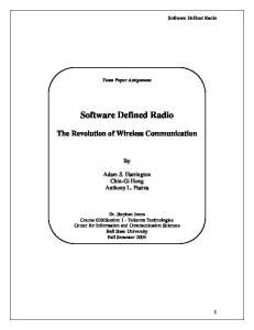
Connect the set-up shown in Figure 1 below.

MASTER SIGNALS

MULTIPLIER

DC

X

AC

SCOPE CH A

DC

Y

100kHz SINE

AC

kXY

100kHz COS

MULTIPLIER

CH B

100kHz DIGITAL 8kHz DIGITAL

TRIGGER

X DC

2kHz DIGITAL 2kHz SINE

Y DC

kXY

Figure 1

This set-up can be represented by the block diagram in Figure 2 below. It generates a 100kHz carrier that is DSBSC modulated by a 2kHz sinewave message.

Master Signals

Message To Ch.A

Multiplier module Y

DSBSC signal To Ch.B

2kHz X 100kHz carrier Master Signals

Figure 2

14.

Adjust the scope’s Timebase control to view two or so cycles of the Master Signals module’s 2kHz SINE output.

15.

Activate the scope’s Channel B input to view the DSBSC signal out of the Multiplier module as well as the message signal.

Experiment 22 – Undersampling in software defined radio

© 2007 Emona Instruments

22-5

16.

Set the scope’s Channel A Scale control to the 1V/div position and the Channel B Scale control to the 2V/div position. Note: The Multiplier module’s output should be DSBSC signal with alternating halves of its envelope forming the same shape as the message.

Question 1 For the given inputs to the Multiplier module, what are the frequencies of the two sinewaves that make up the DSBSC signal?

Question 2 What’s the bandwidth of the DSBSC signal?

17.

Suspend the scope VI’s operation by pressing its RUN control once.

18.

Launch the NI ELVIS Dynamic Signal Analyzer VI.

19.

Adjust the Signal Analyzer’s controls as follows: General Sampling to Run Input Settings 

Source Channel to Scope CHB



Voltage Range to ±10V

FFT Settings

Averaging

  

  

Mode to RMS Weighting to Exponential # of Averages to 3



Markers to OFF (for now)

Frequency Span to 150,000 Resolution to 400 Window to 7 Term B-Harris

Triggering 

Triggering to Source Channel

Frequency Display   

22-6

Units to dB RMS/Peak to RMS Scale to Auto

© 2007 Emona Instruments

Experiment 22 – Undersampling in software defined radio

20.

Verify your answers to Questions 1 and 2 by using the Signal Analyzer’s markers to determine the frequency of the DSBSC signal’s two sidebands.

Ask the instructor to check your work before continuing.

Part B – Direct down-conversion using undersampling If you have successfully completed the experiment on sampling and reconstruction (Experiment 13) you have seen that the mathematical model that defines the sampled signal is:

Sampled signal = the sampling signal × the message

As the sampling signal is a digital signal, the expression can be rewritten as:

Sampled signal = (DC + fundamental + harmonics) × message

When the message signal is modulated carrier like the DSBSC signal that you have set up, the expression can be rewritten as:

Sampled signal = (DC + fundamental + harmonics) × (LSB + USB)

Solving the expression (which necessarily involves trigonometry that is not shown here) gives: 

Duplicates of the LSB and USB (due to their multiplication with sampling signal’s DC component)



Aliases of the LSB and USB at frequencies equal to the sum and difference of their frequencies and the sampling signal’s fundamental frequency



Numerous other aliases of the LSB and USB at frequencies equal to the sum and difference of their frequencies and the sampling signal’s harmonic frequencies

Experiment 22 – Undersampling in software defined radio

© 2007 Emona Instruments

22-7

Recall that the math also proves that, where a low-pass filter is being used to reproduce the original signal by plucking its equivalent out of the sampled signal, the sampling rate must be at least twice the highest frequency in the original signal. If the sampling rate is less than this, aliasing occurs. At first glance then, this suggests that if the DSBSC signal that you have generated is to be sampled, the sampling rate must be at least 204kHz because of the upper sideband is a 204kHz sinewave. However, as the DSBSC signal is bandwidth limited (that is, its spectral composition doesn’t extend down to DC), it’s possible to sample at rates lower than 204kHz without necessarily causing aliasing. For proof, Table 1 shows some of the aliases produced by sampling the DSBSC signal at 150kHz.

Table 1

Components due to DC 98k & 102k

Components due to fs Diff: 48k & 52k Sum: 248k & 252k

Components due to 2fs Diff: 198k & 202k Sum: 398k & 402k

Components due to 3fs Diff: 348k & 352k Sum: 548k & 552k

Notice that none of the aliases overlap the 98kHz and 102kHz components in the sampled signal’s spectral composition. The aliases are either below or above them. So, in this instance, aliasing wouldn’t occur if a band-pass filter (with sufficiently steep skirts) is used to pluck the duplicate of the original DSBSC signal out of the sampled signal. That said, aliasing is still possible by choosing a sampling rate that produces aliases at frequencies that fall inside the band-pass filter’s pass-band. Obviously, as the sampling rate decreases, so too do all of the components in the sampled signal’s spectrum. It makes sense then that, if the right undersampling frequency is used, it must be possible to produce aliases centre on DC. This is crucial because it means that, when a modulated carrier is undersampled, one of its sidebands can be directly down-converted back to a baseband signal without needing to use an intermediate frequency first. All that is needed is a low-pass filter to reject the other aliases. A more sophisticated way of understanding direct down-conversion using undersampling involves thinking of the sampling action as product detection. This is entirely appropriate to do because the math is almost identical – if you’re not sure about that, compare the notes here with the notes in the preliminary discussion on product detection in Experiment 9. The difference is however, instead of multiplying the modulated carrier with a single local sinusoidal carrier, sampling involves multiplying it with dozens of sinewaves (the sampling signal’s fundamental and harmonics). Importantly, as long as one of the harmonics is the same frequency as the modulated carrier, the explanation for a product detector applies equally to undersampling as a form of demodulation.

22-8

© 2007 Emona Instruments

Experiment 22 – Undersampling in software defined radio

To ensure that one of the sampling signal’s harmonics is the same frequency as the modulated carrier, the sampling rate must be a whole integer sub-multiple of the modulated signal’s carrier frequency. That said, to avoid aliasing, the sampling rate must be at least twice the bandwidth limited signal’s bandwidth. The next part of this experiment lets you demodulate your DSBSC signal to recover the 2kHz message using undersampling instead of using a product detector.

21.

Close the Signal Analyzer’s VI.

22.

Restart the scope’s VI by pressing its RUN control once.

23.

Return the scope’s Channel B Scale control to the 500mV/div position.

24.

Modify the set-up as shown in Figure 3 below.

MASTER SIGNALS

MULTIPLIER

DUAL ANALOG SWITCH

CHANNEL MODULE

S/ H

DC

X

S&H IN

AC

S&H OUT

CHANNEL BPF

DC

Y

1 0 0 kHz SINE 1 0 0 kHz COS

2 kHz DIGITAL 2 kHz SINE

SCOPE CH A

kXY

MULTIPLIER

1 0 0 kHz DIGITAL 8 kHz DIGITAL

BASEBAND LPF

IN 1

AC

ADDER

CONTROL 1 CONTROL 2

CH B

NOISE TRIGGER

X DC SIGNAL CHANNEL OUT Y DC

kXY

IN 2

OUT

Figure 3

This set-up can be represented by the block diagram in Figure 4 on the next page. The Multiplier module is used to generate a modulated carrier (DSBSC). The Sample-and-Hold circuit together with the Baseband LPF is used demodulate it using undersampling.

Experiment 22 – Undersampling in software defined radio

© 2007 Emona Instruments

22-9

Under -sampled DSBSC signal To Ch.B

Message To Ch.A

Baseband LPF Y

IN

2kHz

Recovered message

S/ H

X 100kHz carrier

CONTROL

8kHz Master Signals

DSBSC modulator

Demodulation

Figure 4

25.

Compare the undersampled DSBSC signal with the original message. Note: If you look closely, the undersampled DSBSC signal looks a little like an inverted version of the original message.

26.

Modify the scope’s Channel B connection to the set-up as shown in Figure 5 below.

MASTER SIGNALS

MULTIPLIER

DUAL ANALOG SWITCH

CHANNEL MODULE

S/ H

DC

X

AC

S&H IN

S&H OUT

CHANNEL BPF

DC

Y

100kHz SINE 100kHz COS

AC

2kHz DIGITAL 2kHz SINE

BASEBAND LPF

SCOPE CH A

kXY

MULTIPLIER

100kHz DIGITAL 8kHz DIGITAL

IN 1

ADDER

CONTROL 1 CONTROL 2

CH B

NOISE TRIGGER

X DC SIGNAL CHANNEL OUT Y DC

kXY

IN 2

OUT

Figure 5

22-10

© 2007 Emona Instruments

Experiment 22 – Undersampling in software defined radio

Question 3 What’s the significance of the signal on the Baseband LPF’s output?

Question 4 Given the sampling frequency is 8.333kHz (the signal’s specified value of 8kHz is rounded down for simplicity), which harmonic in the sampling signal is demodulating the DSBSC signal?

Ask the instructor to check your work before continuing.

Experiment 22 – Undersampling in software defined radio

© 2007 Emona Instruments

22-11

Part C – Synchronisation Recall that transmitter and receiver carrier synchronisation is essential to successful demodulation using product detection. If the local carrier of a product detector has even the slightest frequency or phase error (relative to the modulated carrier), the demodulated signal is affected. Phase errors can reduce the magnitude of the recovered message and even result its complete cancellation. The effect of frequency errors depends on size. If the error is small (say 0.1Hz) the message is periodically inaudible but otherwise intelligible. If the frequency error is larger (say 5Hz) the message is reasonably intelligible but fidelity is poor. When frequency errors are large, intelligibility is seriously affected. (For a brief explanation of why these effects occur, refer to Part E in Experiment 9.) As direct down-conversion using undersampling is a form of product detection, the sampling signal must be synchronised to the modulated carrier if these effects are to be avoided. The next part of the experiment let’s you see these effects for yourself.

27.

Launch the Function Generator VI.

28.

Adjust the Function Generator for an 8.333kHz output. Note: It’s not necessary to adjust any other controls as the Function Generator’s SYNC output will be used and this is a digital signal.

29.

Disconnect the plug to the Master Signal module’s 8kHz DIGITAL output.

30.

Modify the set-up as shown in Figure 6 below.

FUNCTION GENERATOR

MASTER SIGNALS

DUAL ANALOG SWITCH

MULTIPLIER

CHANNEL MODULE

S/ H

DC

X

S&H IN

AC

ANALOG I/ O

Y

100kHz SINE ACH1

DAC1

ACH0

DAC0

+

CHANNEL BPF

100kHz COS

8kHz DIGITAL 2kHz DIGITAL 2kHz SINE

BASEBAND LPF

IN 1

AC

SCOPE CH A

kXY

MULTIPLIER

ADDER

CONTROL 1

100kHz DIGITAL

VARIABLE DC

S& H OUT

DC

CONTROL 2

CH B

NOISE TRIGGER

X DC SIGNAL CHANNEL OUT Y DC

IN 2

kXY

OUT

Figure 6

22-12

© 2007 Emona Instruments

Experiment 22 – Undersampling in software defined radio

This modification substitutes the Master Signals module’s 8kHz DIGITAL output for an 8.333kHz digital signal from the Function Generator. This allows you to introduce a phase and frequency error between the modulated carrier and the “local carrier” (that is, the sampling frequency’s 12th harmonic).

31.

Observe the effect of this change on the recovered message.

Ask the instructor to check your work before finishing.

Experiment 22 – Undersampling in software defined radio

© 2007 Emona Instruments

22-13