WP/05/27

Exchange Rates in the New EU Accession Countries: What Have We Learned from the Forerunners? Aleš Bulíř and Kateřina Šmídková

© 2005 International Monetary Fund

WP/05/27

IMF Working Paper Policy Development and Review Exchange Rates in the New EU Accession Countries: What Have We Learned from the Forerunners? Prepared by Aleš Bulíř and Kateřina Šmídková1 Authorized for distribution by Marianne Schulze-Ghattas February 2005 Abstract This Working Paper should not be reported as representing the views of the IMF. The views expressed in this Working Paper are those of the author(s) and do not necessarily represent those of the IMF or IMF policy. Working Papers describe research in progress by the author(s) and are published to elicit comments and to further debate.

Estimation and simulation of sustainable real exchange rates in some of the new EU accession countries point to potential difficulties in sustaining the ERM2 regime if entered too soon and with weak policies. According to the estimates, the Czech, Hungarian, and Polish currencies were overvalued in 2003. Simulations, conditional on large-model macroeconomic projections, suggest that under current policies those currencies would be unlikely to stay within the ERM2 stability corridor during 2004–10. In-sample simulations for Greece, Portugal, and Spain indicate both a much smaller misalignment of national currencies prior to ERM2, and a more stable path of real exchange rates over the medium term than can be expected for the new accession countries. JEL Classification Numbers: F31, F33, F36, F47 Keywords: Sustainable real exchange rates, foreign direct investment, ERM2 Author(s) E-Mail Address: [email protected]; [email protected]

1

Aleš Bulíř is thankful for the hospitality of the Czech National Bank. The authors acknowledge the support of colleagues at the NIESR. The paper benefited from comments by Ignazio Angeloni, Jan Babetskii, László Halpern, Katarina Juselius, Jan Kodera, Louis Kuijs, Kirsten Lommatzsch, Martin Mandel, Stanislav Polák, Alessandro Rebucci and participants at seminars at the European University Institute, International Monetary Fund, Prague University of Economics, Czech National Bank, and European Central Bank.

-2-

Contents

Page

I. Introduction............................................................................................................................ 3 II. Forerunners and Latecomers: Are There Lessons to Be Learned?....................................... 4 A. Exchange Rate Developments in the Transition Countries ............................................. 4 B. The Concept of Sustainable Exchange Rates and Accession Countries.......................... 7 III. A Model of FDI-Driven Real Exchange Rates ................................................................... 8 Dynamics around the steady-state ................................................................................ 11 IV. Empirical Evidence........................................................................................................... 13 A. The SRER Model........................................................................................................... 13 B. Forerunners: Test-Driving the Model ............................................................................ 18 C. Computational Results for Sustainable Real Exchange Rates in Accession Countries. 20 V. Policy Implications............................................................................................................. 25 VI. Conclusions....................................................................................................................... 25 Appendixes 1. A Review of Equilibrium Exchange Rate Methodology ................................................ 27 2. The Theoretical Model.................................................................................................... 30 References ............................................................................................................................... 33 Tables 1. Calibrated Elasticity of Export (α) and Import Functions (β).................................. 15 2. Net External Debt Targets........................................................................................ 16 3. Definition of Variables............................................................................................. 17 Figures 1. Latecomers and Forerunners: Selected Indicators, 1991–2003..................................6 2. Capital and Real Exchange Rate Equilibrium.......................................................... 11 3. The Impact of an FDI shock .................................................................................... 12 4. Forerunners: “Smooth Sailing“ During the 1990s, 1992–2003 ............................... 19 5. Latecomers: Misalignment of Real Exchange Rate, 1995–2003.............................. 22 6. Latecomers: How Sustainable Are Current Real Exchange Rates?..........................24 Appendix Tables A.1 Methodologies for SRER Computations................................................................ 28 A.2 Underlying Fundamentals of Medium-term SRERs .............................................. 29

-3-

I. INTRODUCTION The public debate about the adoption of the euro in the new EU accession countries has been framed by three views. First, the euro skeptics argue for opting out. However, all the new accession countries have accepted the obligation of eventual euro adoption. Second, the euro optimists argue that the Exchange Rate Mechanism (ERM2) and the subsequent peg vis-à-vis the euro can be accomplished easily with little or no economic cost. Third, the euro pragmatists’ advice is: “Wait for the right time and the European Central Bank will be flexible in its assessment of euro readiness.” While the skeptics tend to demonize the euro, both the optimists and the pragmatists tend to trivialize the transition cost of euro adoption. This paper attempts to quantify some of those costs. Sustainable real exchange rates (SRERs) are estimated using economic fundamentals. Specifically, we used net external debt, net foreign direct investment (FDI), and domestic and external demand variables. In such a model, real exchange rate appreciation/depreciation manifests itself primarily in larger/smaller accumulation of external liabilities. Just like any model of equilibrium real exchange rates, this approach provides model-specific results that differ from those based on alternative approaches. Model uncertainty remains high in our approach, as the existing literature does not offer a consensual model of equilibrium exchange rate determination. The paper uses the SRER estimates in two ways. First, a gap between the observed real exchange rate and the estimate of the SRER signals a currency misalignment, unsustainable macroeconomic policies, or both. Second, an unstable medium-term SRER projection signals a period of real exchange rate volatility. The authorities can either adjust the exchange rate or, under a fixed regime, adjust macroeconomic policies. Our results indicate a move toward the euro will require either tighter fiscal policies than under the float or much faster GDP and export growth—a continuation of current policies under a peg would result in growing external disequilibria and real exchange rate misalignment. This paper offers several improvements to the existing, predominantly empirical literature on equilibrium real exchange rates. First, we motivate the analysis with a simple dynamic IS-LM framework that underpins real exchange rate developments in countries with large FDI inflows. Second, in the empirical part, we simplify the theoretical model and simulate 2004–09 equilibrium real exchange rate developments conditional on projections from the National Institute Global Econometric Model (NIGEM). Third, unlike most cointegration-based models, our estimates of medium-term misalignment are not mean-reverting, that is, the model allows real exchange rates to depart from equilibrium values during the simulation period of five years. Finally, the robustness of the second-generation SRER model is tested on several forerunners, or current eurozone member countries. Our in-sample simulations of SRERs for those countries that adopted the euro in the late 1990s and early 2000s (Greece, Portugal, and Spain) indicate that they did not have problems with currency misalignment and that the medium-term path of their real exchange rates was fairly stable in the 2000s. In contrast, simulations for some of the new accession countries point to difficulties in entering the ERM2 mechanism too soon after EU entry. Of the four countries we surveyed (the Czech Republic, Hungary, Poland, and Slovenia) all currencies but the Slovenian

-4-

tolar were overvalued significantly in 2003 according to our model. Looking ahead, the model simulations suggest that, under current policies, the currencies would be unlikely to stay within the ERM2 stability corridors during 2004–10, even though they would be converging to their fundamental equilibria. These results suggest that an early “race to the euro” is likely to do more harm than good, unless macroeconomic policies are strengthened. The paper is organized as follows. Section II presents some stylized facts on EU accession countries. Section III outlines a macroeconomic model of real exchange rate and capital stock determination. Section IV shows our empirical results for the second-generation SRER model. Section V suggests some policy implications of our findings, and the final section concludes. II. FORERUNNERS AND LATECOMERS: ARE THERE LESSONS TO BE LEARNED? Historically, European Union (EU) countries, the forerunners, have been put to several tests before being allowed to join the Economic and Monetary Union (EMU), and similar hurdles will have to be overcome by the latecomer countries that joined the EU in May 2004 (Cyprus, the Czech Republic, Estonia, Hungary, Latvia, Lithuania, Malta, Poland, Slovakia, and Slovenia). How challenging is it going to be to meet those conditions for the latecomers? Whereas few problems with euro adoption are foreseen in Cyprus and Malta, a possible conflict between trend appreciation of real exchange rates and the EMU criteria of low inflation and a stable nominal exchange rate is seen in the Central European transition countries. There are, however, other issues at stake than the technical criteria of EMU membership: if a currency were to be irrevocably fixed at an improper parity to the euro, the misalignment would have to be adjusted through other, more costly processes, such as domestic price or wage adjustment. Moreover, locking currencies into an exchange rate regime with the euro too early would remove the shock-absorbing role of monetary and exchange rate policies. Hence, the question can be simplified as follows: is the volatile process of real exchange rate appreciation in the transition countries over, making EMU entry trivial, or is it likely to continue for a few more years, resulting in potentially costly adjustment in those countries? A. Exchange Rate Developments in the Transition Countries Our analysis is motivated by a few stylized facts regarding the transition countries that joined the EU in May 2004, which we will call the “latecomers.” We focus on four of the recent accession countries—the Czech Republic, Hungary, Poland, and Slovenia—for which consistent data and country models are available from the NIGEM.2 First, their currencies have appreciated substantially in real terms during the last decade (Figure 1). On average, between 1992 and 2003, the real exchange rates in the new accession

2

NIGEM is a New-Keynesian macromodel and simulation environment prepared by the National Institute of Economic and Social Research, London. It contains country models of the analyzed accession economies. See Barrell et al. (2002).

-5-

countries appreciated by 3.3 percent annually, one-half of which was realized in 1998–2002.3 Second, most empirical papers agree that rising total factor productivity in the tradable-good sector (the Balassa–Samuelson effect) does not explain fully the gradual and long-lasting real exchange rate appreciation in transition countries (De Broeck and Sløk, 2001, Égert, 2002b, Mihaljek, 2002). A simple version of the Balassa–Samuelson effect implies implausible productivity gains in nontradable good sectors, see, for example, and Flek et al., 2003. Third, the observed appreciation cannot be explained away by the traditional argument of external wealth accumulation (Lane and Milesi-Ferretti, 2000 and 2002). According to that hypothesis, countries with sizable external liabilities need to run large trade balance surpluses to service those liabilities and, consequently, positive net exports require a “competitive,” depreciated real exchange rate. Contrary to the theory, transition economies, with the exception of Slovenia, have piled up external liabilities—their net foreign assets are negative and increasing—and, at the same time, have run persistent trade deficits accompanied by real exchange rate appreciation. Fourth, most transition countries have received massive inflows of foreign direct investment (FDI) that may have affected investors’ perceptions about the countries’ long-term sustainable external balances. Assuming that export growth and productivity improvements are driven by FDI—as compared to competitiveness of national exchange rates—contemporaneous capital inflows may signal expected future net export gains consistent with appreciated real exchange rates. Foreign direct investment is the main culprit in explaining the real exchange rate appreciation, which is otherwise at odds with the observed Balassa–Samuelson and external-wealth accumulation effects. This hypothesis is consistent with previous empirical work related to foreign direct investment in transition countries (Lansbury et al., 1996, and Benáček et al., 2003). Those countries that joined the EU in the 1980s—Greece in 1981 and Portugal and Spain in 1986—and which we will call the forerunners, had had a turbulent past as well. They missed out on early EU entry because their then political regimes made them incompatible with joining and their road to the euro was quite long—20 and 13 years respectively. Prior to adopting the euro, the forerunners appeared to fit a similar pattern of stylized facts as the new accession countries. The forerunners’ real exchange rates appreciated on average by 0.5 percent annually during the ten years prior to joining the EMU, their net external liabilities increased, partly reflecting FDI inflows, and their current account deficits widened.

3

Part of the early real appreciation could be attributable to excessive devaluation at the start of the transition process (Halpern and Wyplosz, 1997).

-6-

Figure 1. Latecomers and Forerunners: Selected Indicators, 1991-2003 140

140

Latecomers: Real effective exchange rates (1991=100) 1/

120

120

Spain

Slovenia

100 80

100 Poland

Hungary

Czech Republic

60

Forerunners: Real effective exchange rates (1991=100) 1/

Portugal

80 60

40

40 1991

20

1993

1995

1997

1999

2001

2003

1991 20

Latecomers: Net foreign assets (In percent of GDP) Slovenia

0

1993

-20

0

1999

2001

2003

Portugal

-40

-40 Hungary

-60

-60

Greece

-80

-80 1991

50

1997

Spain

-20

Poland

1995

Forerunners: Net foreign assets (In percent of GDP)

Czech Republic

60

Greece

1993

1995

1997

1999

1991

2001

50 Hungary

1997

1999

2001

30

Poland l d

Czech Republic

10

Forerunners: Stock of net FDI (In percent of GDP)

40

30 20

1995

60

Latecomers: Stock of net FDI (In percent of GDP)

40

1993

20

Spain

Portugal Greece

10

Slovenia

0

0 1991

15

1993

1995

1997

1999

2001

1991 15

Latecomers: Current account balance (In percent of GDP)

10

Poland

5

10

0

-5

-5 Czech Republic

Hungary

1995

1997

2001

Spain

Greece Portugal

-10

-15

1999

Forerunners: Current account balance (In percent of GDP)

5

Slovenia

0

-10

1993

-15 1991

1993

1995

1997

1999

2001

2003

1991

1993

1995

1997

1999

2001

2003

Source: World Economic Outlook; International Financial Statistics; NIGEM; authors' calculations. 1/ Observations above 100 are defined as an increase in competitiveness, that is, real depreciation vis-àvis the base period.

-7-

B. The Concept of Sustainable Exchange Rates and Accession Countries The concept of a sustainable real exchange rate, which goes back to the research of Artus (1977), can be used for accession-country exchange rate assessment in two ways. First, as a measure of misalignment of historic real exchange rate series.4 Second, as a forward-looking measure of real exchange rate stability in the run-up to euro adoption. The empirical results of real exchange rate misalignment are mixed and often contradictory, depending to a large extent on the method chosen, the two main approaches being single-equation, cointegration-based estimates and normative-target based models (see Appendix I for a review). Authors employing the single-equation, cointegration-based approach assume that the real exchange rate’s return to its equilibrium value is directly observable.5 This might be a reasonable assumption for 30-year-long series of industrial-country exchange rates (Maeso-Fernandez et al., 2001), but it is less so for short, transition-country series that have moved in one direction only (Halpern and Wyplosz, 1997). In contrast, normative-target based estimates originating in the work of Williamson (1994) allow for disequilibrium that is both unobservable from the actual data and long-lasting—real exchange rate developments can be driven by a notional current account or external debt targets. In the group of single-equation estimates, both Halpern and Wyplosz (1997) and De Broeck and Sløk (2001) conclude that the national currencies are significantly undervalued and that equilibrium real appreciation is likely to continue for some considerable time. Frait and Komárek (2001) find that the Czech koruna was appreciated in 1997, but came close to equilibrium thereafter. While Égert (2002a) finds the Czech and Slovak korunas and Polish zloty to be overvalued, in his (2002b) paper the Polish zloty is found broadly in line with the underlying fundamentals. Rahn (2003) presents two alternative models, and although the Czech koruna is overvalued in both, the Polish zloty and Estonian kroon are overvalued in one but undervalued in the other. The puzzling ambiguity was explained by Driver and Westaway (2003), who found that alternative methods of computing equilibrium real exchange rates work with different time horizons and hence most of the differences can be explained away by the horizons of the individual studies. Long-term studies have found transition country currencies typically undervalued, whereas medium-term studies have found them mostly overvalued. By choosing different measures of external equilibrium or different speeds of disequilibrium adjustment, the resulting estimates of real equilibrium rates can change easily. We thus remain doubtful about the policy relevance of results based on the single-equation approach.

4 5

This issue motivated much of the earlier research, see, for example, Isard et al. (2001).

There seems to be a growing cottage industry of cointegration-based, single-currency estimates of real exchange rates. For example, IMF staff published five working papers of this type in the 12 months to May 2003. Similarly, Égert (2003) quotes more than 50 transition-country studies published in the last decade.

-8-

Normative-target based estimates are much less dependent on the horizon of the study, even though they are sensitive to the choice of target variables. At least, and in contrast to the cointegration approach, the sensitivity of exchange rates to the choice of the target variable can be explicitly measured. For example, Spatafora and Stavrev (2003) estimated a model with a current account target, finding that, based on alternative assumptions of the international oil price and trade elasticities, the Russian ruble is either valued fairly or undervalued by up to 40 percent. Coudert and Couharde (2002) based their estimates on current account and output gap targets, concluding that in 2001 the Czech, Estonian, Hungarian, Polish, and Slovenian currencies were all very close to their equilibrium values. Šmídková et al. (2002) estimated a model with a fixed external debt target of 60 percent of GDP for the Czech Republic, Estonia, Hungary, Poland, and Slovenia and found that all currencies but the Slovenian tolar were overvalued in 2000–2001 to the tune of 5–10 percent. The empirical literature to date has focused much less on the issue of real exchange rate stability in the run-up to euro adoption. Égert (2002b) concluded that real exchange rate volatility is not likely to pose a problem and that accession countries should enter the ERM as quickly as possible. Šmídková et al. (2002) were much less optimistic, foreseeing significant volatility unrelated to the underlying fundamentals. We will explore this issue in the empirical section as well. III. A MODEL OF FDI-DRIVEN REAL EXCHANGE RATES In the remainder of the paper we will focus on the role of foreign direct investment and external debt in explaining real exchange rate developments in the new accession countries. 6 To motivate the empirical estimates, we begin by outlining a simple dynamic model of a small, open economy, the real exchange rate developments of which are affected by foreign direct investment. FDI has exercised a powerful effect on transition economies, both by stimulating aggregate supply and by raising permanent income. The two main channels of the impact of FDI on growth are well researched: first, through an increase in total investment and, second, through interaction of the FDI’s more advanced technology with the host’s human capital (Borensztein et al., 1998, and Lim, 2001).7 The literature has offered, however, limited agreement on the quantitative importance of those effects. For the sake of simplicity, we will focus only on the former effect, modeling a positive effect of FDI inflows on net exports (Holland and Pain, 1998).

6

The model does not incorporate any common-currency effect on trade and income (Frankel and Rose, 2002, or Bun and Klaasen, 2002) and the integration of the accession countries with their EU trading partners has already progressed towards the EU levels. Therefore, a common currency itself is not likely to bring a significant integration gain.

7

To the extent the latter channel affects sectoral productivity, it is akin to the Balassa-Samuelson effect.

-9-

In our model—which resembles that of Blanchard (1981)—FDI is equally productive as domestic capital, contributing to capital accumulation. The impact of FDI can be modeled through standard money- and goods-equilibrium schedules, a classical production function, and uncovered interest parity (see also Annex 2). Let us denote them as follows, with lower-case variables representing logarithms: (1) (2)

m − p = αy − β R , y = γk& + δc + ψg + λy * + ρf ,

(LM)

(IS)

where m is the money supply; p is the price level; y and y* are domestic and world output, respectively (y* is external demand unrelated to the real exchange rate); R and R* are the 1 dk domestic and world nominal interest rate, respectively; k is the stock of capital, with k& ≡ k dt and t denoting time; c is the real exchange rate; g is the fiscal impulse; and f is foreign direct investment. Greek characters stand for nonnegative and fixed parameters (all smaller than one).

Output is increasing in the stock of foreign direct investment, f, above and beyond the increase in the capital stock, primarily because FDI generates substantial productivity spillovers outside of its sectoral allocation. The IS curve can be thought of as a demand schedule, while on the supply side physical output is governed by a classical production function: (3)

y = εk ,

where k ≡ i + f , that is, the capital stock, k, is composed of “domestic” capital, i, and “foreign” capital, f, both of which have identical productivity. Capital accumulation is assumed to be decreasing in the existing stock of capital, the real interest rate, and, owing to crowding out, in total debt, d: (4)

⎧k < k * ⇒ k& = οt − θr − φk − ηd ⎨ & ⎩k ≥ k * ⇒ k = ϖt − θr − φk − ηd

We know that countries with a suboptimal capital stock ( k < k * ), that is, latecomers, accumulate capital faster than advanced countries with an optimal capital stock ( k ≥ k * , where k * y * is constant) and, hence, ο > ϖ . Once the capital stock approaches its optimal level, the accumulation process slows down. Total debt is constrained in a debt accumulation schedule, where total debt is accumulated by FDI inflows and fiscal deficits, g, decrease with domestic growth, and, moreover, each

- 10 -

country’s debt is predetermined by its initial level, d :8 (5)

d = d − µy + κf + ιg

In other words, we assume that foreign investors care about the transition country’s growth prospects, return on FDI, and overall prospects of servicing its obligations (Campos and Kinoshita, 2003, and Sethi et al., 2003). It is reasonable to assume that the other commonly used determinants of FDI inflows (lower wages, market attractiveness, “cultural distance,” and so on) are met in the countries in question. The model is closed with uncovered interest parity (6)

e& = R − R * , which can be rewritten in real terms as: c& = r − r * .9

We assume the following relationships between our parameters. First, the direct contribution of FDI to growth (ρ) ought to be larger than the indirect negative impact thereof through larger total debt and capital accumulation (ηκ). Second, the direct growth impact of a fiscal shock (ψ ) is larger than the indirect effect of the capital stock through the production-function-debt nexus ( γηµε ). The solution is a “saddle point” and the equilibrium point is at the intersection of the two stationary lines, k& and c& , in the capital-exchange rate space, with the only convergent path along the dashed line (Figure 2).

8

In another plausible extension of the model, the initial level of debt, d , could be modeled endogenously, with respect to past economic growth, depth of financial markets, and so on. The real exchange rate, c, (c = e + p * − p ) is influenced by world prices, which can be conveniently thought of as fixed. Hence, over time c& = e& − p& and substituting for e& , the path of the real exchange rate is determined by the interest differential c& = r − r * . In this notation, an increase in c implies real depreciation, that is, an increase in competitiveness. 9

- 11 -

Figure 2. Capital and Real Exchange Rate Equilibrium

c . c=0

E

. k=0

k

Dynamics around the steady-state

We consider a few plausible shocks and their impact on the capital stock and real exchange rate. First, an unexpected permanent increase in foreign direct investment will affect both the real exchange rate and the capital stock, as their stationary lines move south, to c&'= 0 and k& ' = 0 respectively (Figure 3.). However, assuming that γκη < ρ , the downward shift in the real exchange rate stationary line is smaller as compared to the capital stock stationary line. As a result, at equilibrium the domestic currency appreciates and the capital stock increases. The real exchange rate appreciation will be instantaneous, with some overshooting, and the capital stock will jump up owing to the FDI shock. Hence, the first round output and net-export effect is ambiguous, depending on the relative size of the real exchange rate and FDI parameters in the IS schedule. Output may even decline, providing the initial loss of competitiveness is large and the increase in capital is small. The stock of capital will continue increasing, however, and, the larger capital stock will boost output, partly offsetting the real appreciation. Needless to say, these features seem to be consistent with the growth pattern of Central European transition countries.

- 12 -

Figure 3. The Impact of an FDI shock

c . c=0 . k=0

. c'=0

E E'

k*

k*'

. k'=0

k

A number of alternative scenarios can be laid out, such as an increase in total debt ( d ) or a permanent increase in foreign demand (y*) (see Annex 2). First, an unexpected increase in the initial level of total debt will affect only the real exchange rate schedule, gradually appreciating the currency and lowering the equilibrium capital stock through FDI outflow. A higher d implies a bigger drain on the external current account and fewer profitable FDI opportunities. Steady-state output declines both because the larger d crowds out future investment (both domestic and foreign) and because the domestic currency appreciates, following the higher interest rates. Second, an unexpected increase in foreign demand has a symmetric impact on the real exchange rate and capital stock schedules through the LM schedule. As a result, both schedules shift down by an equal amount, leaving the steady-state capital stock unchanged and the domestic currency appreciated. Whereas foreign demand raised output, the worsening competitiveness offsets it by the exact same amount. The model above offers a sensible if simplified description of the various channels through which FDI affects the economy. First, we note the additional growth effect from FDI inflows. Second, we observe that the FDI-real exchange rate nexus can dominate the net-foreign-asset nexus of exchange rate determination. Third, the associated real appreciation may offset some of the integration gain. Fourth, the model shows that FDI-dependent economies are vulnerable to changes in their indebtedness.

- 13 -

IV. EMPIRICAL EVIDENCE

We limit the normative-target estimates of sustainable real exchange rates to three forerunners: Greece, Portugal, and Spain, and four latecomers with floating exchange rates: the Czech Republic, Hungary, Poland, and Slovenia. After outlining the empirical model, we rationalize our choice of calibrated parameters, and present the results. The selected approach defines the external balance in terms of stocks rather than flows and emphasizes the role of foreign direct investment as the decisive factor in fundamental-based real exchange rate appreciation. The data are drawn from the NIESR and IMF databases. A. The SRER Model The empirical model

The theoretical model outlined in Section III could be calibrated and simulated, and we would compare the trajectories of debt, trade and other variables under flexible and fixed exchange rates, in two counterfactual exercises. However, we see large benefits of simplifying the framework by treating growth and trade development as exogenous vis-à-vis the model. Rather than exploring the different equilibrating mechanisms under floats and pegs, which are well known anyway, we test how the equilibrium exchange rate would change if the exchange rate regime changed. Is it true, as the pragmatists have argued, that the switch from float to peg should not matter? If it would matter, how serious the resulting real exchange rate misalignment could be? Hence, we take all future macroeconomic variables, such as demand and trade variables, from the NIGEM database as projected under the assumption of flexible exchange rates and focus on a single question: how would the trajectory of the real equilibrium exchange rate change if the nominal exchange rate were to be fixed on January 1, 2004? As explained below, we allow changes to the external debt path and trade flows, but no feedback from real overvaluation to trade developments or growth can take place. Moreover, we allow the misalignment vis-à-vis the equilibrium rate to be long lasting. The normative-target, SRER framework has been built around econometric trade equations relating exports and imports to fundamental variables such as the real exchange rate, the terms of trade, and domestic and foreign economic activity. The SRER model differs from its predecessors in several aspects. First, the FDI-driven integration gains are incorporated directly into the model (Šmídková et al., 2002, and Égert and Lommatzsch, 2003). Second, the current account balance is not restricted, as it is asset and liability stocks, not flows, that define the external equilibrium.10 The sustainable level of external debt is defined according to country specific features, not by a rule of thumb as was done in previous studies. Third, all variables exogenous to the SRER are modeled within an underlying model framework (NIGEM), ensuring consistency and interdependency. 10

This assumption has been popularized by the so-called balance sheet approach, see, for example, Allen et al. (2002).

- 14 Exports increase with the stock of foreign direct investment (FDI) to approximate the integration gain.11 Exports also expand with foreign demand and improvement in the relative price of domestic goods either through real depreciation or a terms of trade change (the real exchange rate being defined in terms of the relative import price): (7)

⎛ EP ⎞ X = α 0 .⎜ m ⎟ ⎝ P ⎠

α1

α1

⎛P ⎞ .⎜⎜ x ⎟⎟ . Y * ⎝ Pm ⎠

( )

α2

.F α3 ,

where X denotes an export index; E is the U.S. dollar nominal exchange rate vis-à-vis the domestic currency; Pm and Px stand for the effective price of imports and exports, respectively; P is the domestic consumer price level; Y* denotes foreign demand; and F measures the FDI-to-GDP ratio. Parameters α1 − α 3 have expected nonnegative values. Demand for imports is driven by domestic activity, the real exchange rate, and the FDI stock: β1

(8)

⎛ EP ⎞ M = β 0 .⎜ m ⎟ .Y β 2 .F β3 , ⎝ P ⎠

where M denotes an import index and Y is domestic output. Parameters β1 and β 2 − β 3 have negative and positive expected values respectively. Moreover, for the integration gain α 3 > β 3 must hold, that is, FDI improves net exports. The trade balance, external borrowing, and net external debt interest payments determine the level of net external debt in any given period. External debt, however, is not an unbounded variable—for a given rate of growth and initial real exchange rate a unique path of sustainable external debt is predetermined. At the same time, accession countries try to exploit fully the maneuvering space of sustainable debt, as FDI inflows bring about the integration gain. In the SRER framework this path can be approximated by considering the initial stock of debt and the country-specific sustainable debt target for the end of the simulation period. To the extent that it is not possible to determine the debt target within the underlying model, we base the targets on selected measures of external sustainability (International Monetary Fund, 2002): (9)

D * = δ [D0 , DT ] ,

where D* denotes the sustainable path of net external debt (in the domestic currency, ratio to GDP), and D0 and DT are the initial and target levels of net external debt. A solution for sustainable real exchange rates reflecting the above economic fundamentals can be found simultaneously using equations (9–11): 11

We hasten to say that our assumption of a positive impact of FDI on the trade balance is not mechanical and the FDI parameter uncertainty is reflected in the size of the confidence interval. The quantitative impact can differ from country to country, depending in the short run on the import component of FDI and in the medium term on whether the new technology produces exportable goods or substitutes for imported goods. Moreover, measurement problems persist in the recording of various FDI components, such as reinvested profits, the impact of FDI on the export price index, and so on.

- 15 -

α1 ⎡ ⎤ β3 β2 * β1 * α1 ⎛ Px ⎞ (10) ⎢ M .β 0 . ( C ) .Y .F − X .α 0 . ( C ) . ⎜ ⎟ .S α 2 .F α3 ⎥ = (1 − r ) D* .Y − D−*1.Y−1 ⎢⎣ ⎥⎦ ⎝ Pm ⎠ where C* is the sustainable real exchange rate; M and X are the volumes of real imports and exports, respectively, in the base year, respectively; and r is the world real interest rate.

Parameter calibration

The parameters used in equation (10) have been calibrated using panel-data results for the five accession countries from Barrell et al. (2002) and Šmídková et al. (2002) (Table 1). We note that, first, the integration gain (α 3 > β 3 ) is statistically significant: a one-percentage point increase in FDI increases net exports by almost 0.5 percent. Second, the FDI elasticities of exports and imports are somewhat higher than the estimates for Ireland, the United Kingdom, Germany, France, Sweden, and the Netherlands.12 Third, the exchange rate elasticity of exports is higher for the latecomer economies than for developed economies alone, reflecting underlying structural and institutional differences between those two groups of countries. Table 1. Calibrated Elasticity of Export (α) and Import Functions (β) 1/ Parameter and its notation

Value

Export Function (7) Real exchange rate elasticity of exports

α1

3.15

Foreign demand elasticity of exports

α2

1.00*

FDI (stock) elasticity of exports

α3

0.70

Real exchange rate elasticity of imports

β1

-0.62

Domestic demand elasticity of imports

β2

1.00*

FDI (stock) elasticity of imports

β3

0.24

Import Function (8)

Source: Šmídková et al. (2002). 1/ Parameter values denoted with an asterisk were imposed during the estimations to ensure that the country’s share of world exports and imports is independent of both the level of world trade and domestic demand.

12

See Barrell and te Velde (2000) and Pain and Wakelin (1998).

- 16 The paper incorporates a trade-based, country-specific definition of external balance (Table 2), whereas the earlier models assumed a rule of thumb, end-period net external debt target equal to 60 percent of GDP for all countries (Ades and Kaune, 1997). Recent events in emerging economies have shown that the rule-of-thumb approach may not be flexible enough and that sustainable external debt ought to be related to countries’ ability to service it (International Monetary Fund, 2002). Uncertainty related to the sustainable external target can be large. Nevertheless, the impact of changes in the sustainable debt-to-GDP ratio on the SRER estimates is relatively insignificant: a 10-percentage point change in the ratio generated a change in the equilibrium real exchange rate of 0.04–0.4 percent only (Šmídková et al., 2002). We employ the following target levels of net external debt, which are binding in 2022: Table 2. Net External Debt Targets Country The Czech Republic, Hungary, Slovenia Poland, Greece, Portugal, Spain

Exports-to-GDP Ratio (in percent)

External Debt Target

Higher than 40

65

Higher than 30, but lower than 40

53

Source: Authors’ calculations based on International Monetary Fund (2002). Data issues

Data consistency is crucial for SRER calculations, given the endogenous relationship between various variables, such as domestic and foreign demand or trade and financial flows. We rely on the global econometric model (NIGEM) maintained by the National Institute of Economic and Social Research, which allows us to project domestic and external within the same model (Table 3). Our model experiment is based on an unconditional forecast—we implicitly assume that the NIGEM projection represents the optimal trajectory of macroeconomic developments.

- 17 Table 3. Definition of Variables Variable Effective foreign import demand (in millions of US dollars) Effective world real interest rate (in percent) Import prices (index) Export prices (index) US dollar exchange rate (in domestic currency terms) Real domestic output (in constant prices) Real exports (base index) Real imports (base index) Domestic consumer price index (CPI) Export volume in the base year (1994) (in millions of US dollars) Import volume in the base year (1994) (in millions of US dollars) Initial level of external debt (in millions of US dollars) Stock of FDI (in percent of GDP)

Notation

Data Source

S

NIGEM, February 2004

r Pm Px

NIGEM, February 2004 NIGEM, February 2004 NIGEM, February 2004

E

NIGEM, February 2004

Y X M P

NIGEM, February 2004 NIGEM, February 2004 NIGEM, February 2004 NIGEM, February 2004 IMF, Balance of payments Statistics Yearbook, 2002 IMF, Balance of Payments Statistics Yearbook, 2002 NIGEM, February 2004; IFS; and Rider (1994) 1/ NIGEM, February 2004; IFS; and Rider (1994) 1/ Calculations based on International Monetary Fund (2002)

X M D0 FDI

Net external debt target for time T (T = 2022; in D* percent of GDP)

1/ Calculations based on NIGEM projections of FDI flows and initial estimates of the FDI stock consistent with the estimate of the initial stock of net foreign assets (NFA).

Simulation techniques and result uncertainty

We solved equations 7–10 in the WinSolve 2.0 simulation package, using the Newton procedure. Most data are derived from the NIGEM database, while some historical series we supplanted with IFS data. For off-sample simulations NIGEM projections were also used. Hence, the only variable simulated in equation (10) is the sustainable real exchange rate. All other projected variables are treated as exogenous vis-à-vis our model. For each country, baseline SRERs are calculated by solving equation (10) using the Newton procedure for the period 1995Q1:2010Q4 in WinSolve (2003). Input variables are set equal to the observed values for the in-sample computations (1995Q1–2003Q4) and to the forecasted values for the out-ofsample computations (2004Q1–2010Q4). As with all simulations, the SRER estimates are useful only to the extent that we can be confident about their significance. Economists are generally faced with two basic uncertainties. While parameter uncertainty is reflected in the width of the confidence interval, the more serious of the two, model uncertainty, is best addressed by applying the model to different

- 18 countries and/or periods. We performed both extensive sensitivity tests and comparisons with other papers assessing the real exchange rates of accession countries. Regarding the former, confidence intervals are calculated for both the in-sample and off-sample (projection) periods. While the in-sample confidence intervals are simulated using the estimation errors of the trade equations, the off-sample confidence intervals are based on the historical standard errors of the exogenous variables and the uncertainty about the target value of the external debt (D*). As far as the precision of our estimates is concerned, we found confidence bands of a similar order as compared to other studies on fundamental real exchange rates.13 Regarding model uncertainty, we compared our results with recent medium-term studies and found that our estimates of misalignment were of similar sign and magnitude (Égert and Lommatzsch, 2003).14 We acknowledge, however, that the current literature offers no definitive way of determining the true model of equilibrium real exchange rates. B. Forerunners: Test-Driving the Model

Before applying our framework to the new accession countries, we tested the model on the sample of the three forerunners: Greece, Portugal, and Spain. The Portuguese escudo and Spanish peseta started the two-year pre-adoption period in 1996, whereas the Greek drachma started in 1998.15 Following a two-year period of nominal-convergence assessment, these countries adopted the euro in 1999 and 2001, respectively. We ask the following question: did the change in exchange rate regime affect external equilibrium and cause misalignment?16 To answer this question, we simulate equation 10 using the relevant data, obtaining an estimate of the real equilibrium exchange rate as well as estimates of the confidence intervals, called the SRER corridor. We find that, first, all forerunners started their ERM membership with fundamentally correct parities vis-à-vis the euro and, second, prior to euro adoption, after two years in the ERM, their parities appeared sustainable (Figure 4). Regarding the former, the peseta was slightly undervalued and the drachma and escudo were within their SRER corridors. Regarding the latter, the drachma remained broadly in line with the equilibrium rate predicted by the model,17 whereas the euro was some 10–20 percent too strong in real terms for Portugal and Spain, 13

Williamson (1994) and Bayoumi, Clark, Symansky, and Taylor (1994) report alternative estimates of the uncertainties pertaining to computations of equilibrium real exchange rates. Detken et al. (2002) estimate the uncertainty specifically for the equilibrium real exchange rates of the euro at around 20%. 14

More detailed results of sensitivity tests are available from the authors upon request.

15

To be exact, the peseta and escudo were floated against the euro in 1989 with special 6-percent fluctuation bands.

16

Besides being interesting per se, this exercise was a useful test of the underlying model, confirming that the calibrated model fits the trade performance of the forerunners reasonably well.

17

It is worth remembering that Greece took full advantage of two rather unique circumstances. First, as a result of pressures following the Asian crisis, it joined ERM2 with a central parity some 12 percent weaker than the market rate at that time. Second, the central bank was subsequently able to engineer a steady depreciation of the market rate.

- 19 Figure 4. Forerunners: “Smooth Sailing” During the 1990s 1/ 1.3

Greece

1.2

Narrow stability corridor

SRER corridor

1.1

REER

1.0 0.9

Wide stability corridor

0.8 1992q1 1.3

1993q3

1995q1

1996q3

1999q3

2001q1

Wide stability corridor

Spain

1.2 1.1

1998q1

2002q3

Narrow stability corridor

REER

1.0 SRER corridor

0.9 0.8 1992q1 1.3

1993q3

1995q1

Portugal

1996q3

1998q1

1999q3

Wide stability corridor

1.2

2001q1

2002q3

Narrow stability corridor

1.1 1.0

SRER corridor

0.9 REER 0.8 1992q1

1993q3

1995q1

1996q3

1998q1

1999q3

2001q1

2002q3

Source: Authors’ calculations. 1/ The narrow and wide bands are defined as 3.75 percent and 16.5 percent, respectively, around the central estimate during the ERM. The band is narrowed to 1.5 percent thereafter, as the national exchange rates are fixed and only the inflation criterion matters. 1994 = 1.

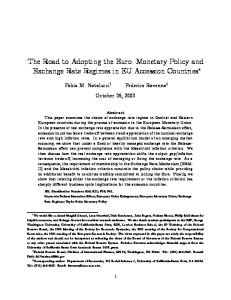
- 20 reducing their competitiveness. In summary, the model indicates that the forerunners entered both the ERM and the eurozone at the right time and with the right parity. Post-adoption real appreciation vis-à-vis the SRER, however, seemed to be relatively persistent, with no signs of abating. These findings seem broadly consistent with the recent trade and especially debt developments in the forerunner countries (see, for example, International Monetary Fund, 2004). What does the forerunners’ “smooth sailing” in the run-up to euro adoption imply for the latecomers’ entry into the eurozone? The results will depend on two issues. First, on the initial real exchange rate misalignment and, second, on the volatility of the latecomers’ macroeconomic forecasts vis-à-vis the actual developments in the forerunner group. On the one hand, the forerunners’ historic real exchange rate volatility was only 0.1 percent, as against 3.3 percent in the latecomer countries, mostly as a result of tightly managed nominal exchange rates in the run-up to euro adoption. On the other hand, the average export-to-GDP ratio in the Czech Republic, Hungary, and Slovenia is almost 60 percent, as compared to less than 30 percent in Greece, Portugal, and Spain, presumably lowering the exchange rate volatility. Moreover, Portugal and Spain entered the ERM in 1996 during a period of relative tranquility on international financial markets. We also noticed some surprising post-ERM developments in the forerunner countries that would have interesting implications for the latecomers. First, the stock of net FDI declined following the adoption of the euro, in part owing to a slowdown in FDI inflows (Figure 1). Should an FDI slowdown occur in the latecomer countries, it would generate two processes. On the one hand, it would depreciate the equilibrium exchange rate even more, hence, increasing the misalignment and making entry into the eurozone more difficult. On the other hand, it would limit the expected integration gain, restricting real convergence. Second, the adoption of the euro accelerated the forerunners’ accumulation of foreign liabilities (Figure 1), which was possible because the stock of external debt was initially low and certainly lower than in the latecomer countries at present. C. Computational Results for Sustainable Real Exchange Rates in Accession Countries

In this section, we will provide two sets of empirical results for the Czech koruna, Hungarian forint, Polish zloty, and Slovenian tolar. First, a measure of the misalignment of real exchange rates. Second, a forward-looking measure of real exchange rate stability in the run-up to euro adoption, conditional on NIGEM macroeconomic forecasts. The results of these tests— conditional on NIGEM macroeconomic projections—are not commensurate with early ERM2 entry.

- 21 Misalignment

We find that three out of the four accession currencies were significantly above their fundamental-based equilibrium exchange rates in 2003 (Figure 5). Fixing the euro conversion rates at the early-2004 exchange rates and without major policy adjustments to reverse the slide in fundamentals would have posed a major problem for the forint, zloty, and koruna (in that order), but not for the tolar. Even if we disregard the numerical values of the estimated misalignment—our estimates have fairly wide confidence intervals and depend on post-2004 projections of macroeconomic variables—the recent developments signal a significant break with the past. On average, the fundamentals explained about 60 percent of the real appreciation during the last decade. We can only conjecture what might explain the rest. Some obvious culprits include excessively optimistic expectations about the speed of real and nominal convergence, a temporary impact of privatization inflows, and the psychological effect of EU enlargement. It may be that the exchange rate correction that took place during 2003 marks the start of less optimistic assessments of the new accession countries. And part of the misalignment is possibly due to medium-term volatility of nominal exchange rates. The Czech koruna. Following the 1997–1998 currency turmoil, the koruna was allowed to float under an inflation-targeting regime. From a minor undervaluation during 1995–1997, owing to a low level of indebtedness, the koruna appreciated sharply in 1999 to 5 percent above its fundamental-based value. The overvaluation increased to about 15 percent at end-2003, owing to accumulation of external liabilities, although part of the misalignment was corrected through nominal depreciation. The simulated confidence band was narrow at ±5 percent. The Hungarian forint. Although the real exchange rate of the forint was more volatile than the other currencies in our sample, it remained close to its equilibrium value until end-2000, mostly owing to the tight crawling peg pursued by the National Bank of Hungary. Although net foreign assets were improving, recorded FDI declined. Starting in 2001, the central bank put more emphasis on price stability and less on exchange rate stability, resulting in a massive appreciation of the forint equivalent to almost 50-percent misalignment at mid-2003. In late 2003, this disequilibrium was corrected partly. The confidence band was wide at ±11 percent. The Polish zloty. The Polish currency was close to its fundamental value until early 2000, thanks to its crawling-peg regime. Following a change in the monetary policy regime in 1999, gradual real appreciation led to a misalignment of some 15–25 percent in 2002. Similar to the Czech Republic, the accumulation of external liabilities has increased recently. In 2003, the zloty depreciated and the currency misalignment was reduced to below 20 percent at the end of the year. The confidence band was narrow at ±4 percent. The Slovenian tolar. After a protracted period of real undervaluation, the tolar seemed to be in line with its fundamentals at the end of 2003. The confidence band was narrow at ±3 percent. Interestingly, Slovenia is the only accession country in our sample that did not rely on exchange-rate stabilization, even though official guidance of the exchange rate has been considerable (Borghijs and Kuijs, 2004), and that did not fully liberalize its financial account.

- 22 -

Figure 5. Latecomers: Misalignment of Real Exchange Rates, 1995-2003 (Deviation from the estimated SRER, in percent) 60

60

Czech Republic

Hungary

40

40

20

20

0

0

-20

-20

-40

-40

1995q1

1997q1

1999q1

2001q1

2003q1

60

1995q1

1997q1

1999q1

2001q1

2003q1

1999q1

2001q1

2003q1

60

Poland

Slovenia

40

40

20

20

0

0

-20

-20

-40

-40

1995q1

1997q1

1999q1

Source: Authors' calculations.

2001q1

2003q1

1995q1

1997q1

- 23 -

Sustainability

We find that in our model the nominal convergence required by the Maastricht criteria and ERM2 may prevent the forint, koruna, and zloty—at their end-2003 levels—from converging toward their equilibrium real exchange rates. In other words, fixing those currencies and assuming six more years of current macroeconomic policies—as projected by NIGEM—would still not guarantee the achievement of fundamental equilibrium. Thus, floating-regime policies would not be good enough for fixed-regime environment of the ERM2. Formally, we compare the estimated SRER confidence bands with the so-called “stability corridors” that are to reflect the convergence criteria for both for inflation and exchange rate stability (Figure 6).18 For the period 2004–2010 we find the SRERs appreciating in all four countries, but the koruna and forint appear to be the farthest away from the implied ERM2 corridor and, hence, at odds with the ERM2 entry date toward the end of the decade.19 As a result of their end-2003 misalignment, both currencies remain well outside the narrow 3 3 ⁄4 -percent stability corridor throughout 2010. Only in the late 2000s would the mid-point of the estimated koruna SRER approach the wider, 16 1 ⁄2 -percent stability corridor. The mid-point of the forint SRER would be some 30 percent above the upper band of the wider corridor. The results for the tolar suggest the opposite scenario—it would need a modest revaluation toward the end of the decade. The zloty is the only currency where our calculations suggest end-period convergence of the SRER and stability corridors, that is, ERM2 entry seems consistent with the pre-announced date. The Czech koruna. During 2004–2010 the nominal convergence criteria will be too restrictive to bring the domestic currency into line with the external balance. The koruna at the end-2003 exchange rate will remain overvalued, as the fundamental-driven appreciation will not be fast enough to compensate for the initial misalignment. The Hungarian forint. During 2004–2010 the nominal convergence and external balance are found to be incompatible at the end-2003 exchange rate. The Polish zloty. During 2004–2010 the zloty follows a path similar to the koruna, only faster. In the short-term, the nominal convergence criteria will be too restrictive to bring the zloty into line with the external balance. Toward the end of the decade both corridors begin to overlap, signaling that nominal convergence may be sustainable at the end-2003 exchange rate.

18

ERM2 permits nominal exchange rate fluctuations within a ±15 percent band. This requirement differs from the exchange rate stability criterion, which requires “observation of the normal fluctuation margins provided by the exchange-rate mechanism of the European Monetary System, for at least two years, without devaluing against the currency of any other Member State” (Article 121(1) of the Maastricht Treaty). Specifically, the criterion was set as fluctuation margins of ±2 ¼ percent against the median currency (EC Convergence Report 2000, Annex D).

19

The date pre-announced by the Czech, Hungarian, and Polish authorities is based, however, on the fiscal Maastricht criteria, namely that of an overall fiscal deficit of no more than 3 percent of GDP. Equilibrium exchange rate calculations were not a part of this decision.

- 24 Figure 6. Latecomers: How Sustainable Are Current Real Exchange Rates? 1/ 2.0

2.5 Czech Republic

Hungary SRER corridor

1.5

2.0

Narrow stability corridor 1.0

Wide stability corridor

SRER corridor

REER 1.5

Narrow stability corridor

REER

Wide stability corridor

1.0

0.5 1995q1 1997q3 2000q1 2002q3 2005q1 2007q3 2010q1

1995q1 1997q3 2000q1 2002q3 2005q1 2007q3 2010q1

2.0

2.0

Poland

Slovenia

1.5

1.5 Narrow stability corridor SRER corridor

REER 1.0

1.0

Narrow stability corridor

Wide stability corridor

SRER corridor REER

Wide stability corridor

0.5 1995q1 1997q3 2000q1 2002q3 2005q1 2007q3 2010q1

0.5 1995q1 1997q3 2000q1 2002q3 2005q1 2007q3 2010q1

Source: Authors’ calculations. 1/ The narrow and wide bands are defined as 3.75 percent and 16.5 percent around the central estimate respectively, to reflect both the inflation (1.5 percent) and exchange rate (2.25 percent) convergence criteria. 1994 = 1.

- 25 The Slovenian tolar. During 2004–2010 the nominal convergence appears sustainable with respect to the external balance. However, a revaluation of up to 20 percent might be needed toward the end of the period. In summary, our model findings suggest that if those four countries were to enter the ERM2 in 2004 and try to meet Maastricht criteria as well under the existing, floating-regime macroeconomic policies, it might do them more harm than good. At present, all currencies but the tolar seem to be overvalued and are likely to remain so for a considerable time. V. POLICY IMPLICATIONS

According to our model, early adoption of the euro by the latecomer countries is unlikely to be as smooth as that by the forerunner countries given current macroeconomic policies. At end-2003, just before EU enlargement, real exchange rates were not close to their fundamental-based values and an early fixing vis-à-vis the euro would have resulted in a overvalued currencies in all countries but Slovenia. From a medium-term perspective, meeting the convergence tests for exchange rate and price stability would be costly, owing to the only gradual convergence of equilibrium real exchange rates toward the narrow band. What would need to be done to achieve convergence in our model? Either the new accession countries’ growth and export performance would have to improve substantially compared to our model or their macroeconomic policies—fiscal deficits and external debt—would have to be tightened compared to the NIGEM projections under flexible exchange rates (Schadler et al., 2004). In other words, what we paraphrased as the pragmatist approach—wait for the right time and do what you can—may not be a viable option. While this approach served some countries well in the past—most notably Greece—it may not work for the new EU accession countries, given the simulated slow adjustment of their exchange rates to fundamental equilibrium and large initial disequilibria. Moreover, increased uncertainty may be a problem: finding the “right” time and the “right” exchange rate is likely to be more difficult than in the past. Our results also suggest that following the adoption of the euro, the convergence problems would not disappear. For example, should a slowdown of FDI inflows—similar to that in the forerunner countries—materialize, the latecomers’ real convergence might decelerate substantially. Moreover, it is unclear whether the new EU accession countries would be able to accumulate foreign liabilities in a fashion comparable to the forerunners, given their already high levels of external debt. Although external financing of fiscal deficits has been modest to date, as the fiscal deficits in the Czech Republic, Hungary, and Poland continue to swell, their governments are likely to start competing with the private sector for external financing. VI. CONCLUSIONS

This paper develops a theoretical model of real exchange rate determination with strong neoclassical effects, and simplifies and simulates it on a sample of three “forerunners” and four new accession countries using time series from the NIGEM database. The observed real exchange rates are then compared with simulated real equilibrium exchange rates based on the assumption that the nominal rates to the euro were fixed at a certain point in time. Unlike in most other models, the resulting misalignment can be long lasting, as we do not impose mean reversion.

- 26 -

The simulations of the sustainable real exchange rates (SRERs) in four of the new accession countries suggest that three of them (the Czech Republic, Hungary, and Poland) would likely experience difficulties during their stay in the ERM2 mechanism if they joined too early. According to our results, all currencies but the Slovenian tolar were overvalued in 2003. Simulating the performance of SRERs through to 2010, we find that the currencies fixed at their end-2004 exchange rates would likely not stay within their stability corridors, conditional on NIGEM macroeconomic projections. The primary impact of external disequilibrium in this model is accumulation of debt and erosion of external competitiveness. Pursuing the convergence criteria too soon may harm the competitiveness of the Czech, Hungarian, and Polish economies, while the Slovenian currency may require revaluation prior to euro adoption. In contrast, ex post simulations for those countries which accepted the euro in the late 1990s—Greece, Portugal, and Spain—show no real exchange rate misalignment of their national currencies at that time. Moreover, their real exchange rates followed a more stable, medium-term path than can be expected in the new accession countries. An early “race to the euro” may be a costly competition indeed.

- 27 -

APPENDIX I

A Review of Equilibrium Exchange Rate Methodology

New methodological and empirical studies tend to emerge every time changes in exchange rate regimes are debated. For example, the debate of the early 1990s motivated a rich branch of literature. Barrell and Wren-Lewis (1989) computed fundamental equilibrium exchange rates for the G-7 group. Artis and Taylor (1993) proposed a concept of desired equilibrium exchange rates reflecting fiscal policy targets. Williamson (1994) compared several approaches to estimating equilibrium exchange rates. Stein and Allen (1995) described fundamental determinants of real exchange rates. MacDonald (1999) emphasized the distinction between long-run and short-run fundamentals. In these benchmark studies, the outcomes of computations are often called equilibrium real exchange rates. Adjectives such as fundamental, desirable and behavioral emphasize various methodological specifics. Alternative SRER concepts take different approaches to the role of economic policies and to the selection of economic fundamentals. SRERs also assume different concepts of equilibrium. Driver and Westaway (2003) explain how alternative methodologies work with different time horizons, the three main approaches being single-equation, typically cointegration-based estimates, normative-target based models, and general equilibrium models. These relate to short-, medium-, and long-term horizons, respectively. We suggest that the medium-term concept is the most suitable for analyzing real exchange rates in the accession countries, in particular given the time span of their entry into the euro area. More recently, the policy debate in the new accession countries spawned numerous empirical studies. All these studies are rooted in some way in the original debate outlined above. Equilibrium real exchange rates were initially estimated for industrial countries (Artis and Taylor, 1993; Feyzioğlu, 1997), and subsequently extended to developing countries (Elbadawi and Soto, 1997; Mongardini, 1998; and MacDonald and Ricci, 2003) and to transition economies (Halpern and Wyplosz, 1997; De Broeck and Sløk, 2001; Égert, 2002a and 2002b; Frait and Komárek; 2001, Rahn, 2003; and Spatafora and Stavrev, 2003). The SRER concept was suggested in Šmídková, Barrell, and Holland (2002), who argued that it better reflects some specific features of the former transition economies, namely their FDI-driven convergence and relatively large current account deficits.20 The resulting estimates depend to a large extent on the methodology chosen. The SRER approach is equivalent to a medium-term methodology working with a macroeconomic specification of real exchange rates (Table A.1).21 These normative-target estimates follow the

20

Barrell et al. (2002) describes the underlying macroeconomic models estimated for the accession economies on panel data.

21

Other methodologies work with sector specifications, based on relative prices of tradable and nontradable goods. The sector approaches cannot be used for assessing the relative price of the domestic currency vis-à-vis the euro and therefore are not included in our survey.

- 28 -

APPENDIX I

work of Williamson (1994), who searched for a medium-term equilibrium unobservable from the actual data. According to this approach, real exchange rate developments can be driven by notional current account or external debt targets. The medium-term models do not necessarily reflect equilibrium on all asset markets, since some of the markets do not clear in the medium term due to various adjustment costs. As a result, stock variables, such as NFA and stock of FDI, only converge to their long-term equilibrium levels. In contrast, the short-run empirical models assume that the equilibrium real exchange rate trajectory can be observed directly. Consequently, they typically find smaller currency misalignments than the medium-term models. Their estimates of short-term real misalignment are determined mainly by financial market developments. Finally, long-term equilibrium exchange rate models are rooted in general equilibrium theory and show the total impact of real convergence on exchange rates. These models often find different estimates of real misalignment from the medium-term SRERs. Unfortunately, the long-term dynamic general equilibrium models are defined as deviations from equilibrium values and, hence, cannot be used to compute the levels of equilibrium real exchange rates. Table A.1 Methodologies for SRER Computations 1/ Horizon/Model

Short-term horizon

Structural model, theoretical assumptions Empirical estimates, reduced forms, panels

NATREX 2/ BEER

Medium-term horizon FEER DEER FRER

Long-term horizon NATREX PPP Large panels with longterm fundamentals

1/ The various SRER concepts are explained in the following studies: fundamental equilibrium exchange rates (FEER) in Williamson (1994); desirable equilibrium exchange rates (DEER) in Artis and Taylor (1993); fundamental real exchange rates (FRER) in Šmídková, Barrell, and Holland (2002); the natural real exchange rate (NATREX) in Stein and Allen (1995); purchasing power parity (PPP) in Williamson (1994); and the behavioral equilibrium exchange rate (BEER) in MacDonald (1997). An example of a large-panel approach can be found in Halpern and Wyplosz (1997). 2/ The NATREX can be either estimated from a reduced form of an underlying model or computed directly from this model. In the first case, the results are similar to those of the short-run approaches. Applications of the latter approach are relatively rare (Detken et al., 2002).

Medium-term SRERs are usually computed with the use of a larger underlying macroeconometric model. It is quite common to assume that the full employment line is vertical with respect to the real exchange rate and to compute SRERs from the trade equations of the underlying model and from an added identity for the external balance. The underlying model can also be used to produce scenarios for variables exogenous to the trade equations. Due to the different structures of the underlying models, different SRERs give emphasis to different economic fundamentals (Table A.2). For example, the role of FDI is only accentuated by the FRER model.

- 29 -

APPENDIX I

Table A.2 Underlying Fundamentals of Medium-term SRERs SRER concept/ Set of fundamentals External trade (terms of trade, domestic and foreign demand) International assets (world interest rate) Internal balance (vertical full-employment line) External balance (current account target, debt target) Convergence factors (determinants of real appreciation) 1/ Other policy-relevant factors

FEER

DEER

FRER

Yes

Yes

Yes

Yes

Yes

Yes

Yes

Yes

Yes

Current account target

Current account target

External debt target

Sustainable capital inflows

Sustainable capital inflows

Stock of FDI (integration gain)

None

Fiscal policy target

Initial level of debt

1/ The “convergence factors” are variables that help to explain why a relatively fast real appreciation of exchange rates and current account deficits can be sustainable. Specifically, if a country obtains a significant portion of capital inflows that are evaluated by the financial markets as sustainable, larger current account deficits are possible without increased risks of exchange-rate crisis. Analogously, an increasing stock of FDI implies that a host country can benefit from the “integration gain”, and consequently from a stronger currency, without additional costs.

We find two major differences between the FRER concept and other SRERs. The FRER defines the external balance in terms of stocks rather than flows and emphasizes the role of FDI as the decisive factor in fundamental-based real exchange rate appreciation. Both characteristics are typical for accession economies and are difficult to capture in other models. Moreover, the FRER employs a less binding definition of the external balance, allowing comparatively high current account deficits during the pre-EMU period when the catch-up process is likely to be the fastest. However, temporarily larger current account deficits are only sustainable to the extent of the normative debt target. Both approaches, FRER and SRER, depend on the international environment—a shock to capital flows would change the path of the equilibrium exchange rate.

- 30 -

APPENDIX II

The Theoretical Model

Consider a small, open economy described by standard money- and goods-equilibrium schedules, a classical production function, and the uncovered interest parity relationship: m − p = αy − β R

(LM)

y = γk& + δc + ψg + λy * + ρf ,

(IS)

y = εk ,

(Classical production function)

where k ≡ i + f e& = R − R *

(Uncovered interest parity)

and hence in real terms: c& = r − r * ⎧k < k * ⇒ k& = οt − θr − φk − ηd ⎨ & ⎩k ≥ k * ⇒ k = ϖt − θr − φk − ηd

(Capital accumulation schedule)

d = d − µy + κf + ιg

(Debt accumulation schedule)

where m is the money supply; p is the price level; y and y* are domestic and world output respectively; R and R* are the domestic and world nominal interest rate respectively; k is the stock of capital; c is the real exchange rate; g is the fiscal impulse; f is foreign direct investment; d is the real stock of total debt, both public and private; d is an initial level of real debt; and t is time. Greek characters denote positive and fixed parameters (all smaller than one) and variables with a star denote world variables. All lower-case variables are in logarithms. The model has the following exogenous variables: p*, R*, g, y*, f, d , and t; endogenous variables: y, m, R, e, p, and d; and state variables: c and k, where c is the driving (jump) variable and k is the predetermined variable. Substituting from the LM schedule into the uncovered interest parity we obtain: 1 e& = (αεk − m + p ) − R * and rearranging the IS schedule yields:

β ε δ ψ λ ρ k& = k − c − g − y * − f . From the capital accumulation schedule we find the γ γ γ γ γ

expression for the real interest rate in transition and advanced countries respectively: r=−

[

1 & k − οt + (φ − ηµε )k + ηd + ηκf + ηιg

θ

]

- 31 -

APPENDIX II

and r=−

[

]

1 & k − ϖt + (φ − ηµε )k + ηd + ηκf + ηιg .

θ

Finally, substituting for r and k& in the real exchange rate relationship we obtain for the transition country:22 ⎛ ρ ηκ ⎞ ⎛ ψ ηι ⎞ ⎛ ε φ ηµε ⎞ δ η λ ο c& = ⎜⎜ − y * +⎜⎜ − ⎟⎟ f + t − R * . ⎟⎟k + c − d + ⎜⎜ − ⎟⎟ g + − + θ ⎠ γθ θ γθ θ ⎝ γθ θ ⎠ ⎝ γθ θ ⎠ ⎝ γθ θ The state-variable relationships can be expressed in a matrix: ⎡ δ ⎡ c& ⎤ ⎢ γθ ⎢k& ⎥ = ⎢ δ ⎣ ⎦ ⎢− ⎢⎣ γ

γηµε − ε − γφ ⎤ ⎡ ρ − γηκ ⎥ ⎡ c ⎤ ⎢ γθ γθ ⎥⎢ ⎥ + ⎢ ε ⎥ ⎣k ⎦ ⎢ − ρ ⎥⎦ ⎢⎣ γ γ

ψ − γηι γθ ψ − γ

−

η θ

0

λ γθ λ − γ

ο θ 0

⎡ f ⎤ ⎢ ⎥ ⎤⎢ g ⎥ − 1⎥ ⎢d ⎥ ⎥⎢ ⎥ 0 ⎥ ⎢ y *⎥ ⎥⎦ ⎢ t ⎥ ⎢ ⎥ ⎣⎢ R *⎦⎥

⎛ ⎞ δψ δηµε + < 0 ⎟⎟ as long as the output The determinant of the Jacobi matrix is negative ⎜⎜ ∆ = − γθ γθ ⎝ ⎠ effect of a fiscal shock is large compared to the indirect output effect of a capital stock shock through the output-debt nexus (ψ > ηµε ) . Hence, the solution to the dynamic system is a saddle point with the usual properties and the motivation of a “rational-expectations” equilibrium.23 We can easily obtain the slopes of the exchange rate and capital stock stationary lines: dk dc

c& =0

=

δ ε + γφ − γηµε

> 0 and

dk dc

k& =0

=

δ >0. ε

Under the assumptions spelled out earlier, the absolute value of the latter one is larger and, hence, k& = 0 is flatter as compared to the former (δ / ε > δ / (ε + γφ − γηµε )) . From the Jacobi matrix we determine that the only convergent path under the saddle-path solution is along the dashed line.

22 23

For simplicity, we show only the solution of the transition-country version of the model.

Strictly speaking, given the presence of time in our capital accumulation schedule, the equilibrium point shifts over time. For the sake of simplicity, we ignore this issue.

- 32 -

APPENDIX II

The schedule shifts as a result of the FDI, debt, and foreign demand shocks, respectively, as discussed in the text are: ∂c ∂f ∂c ∂d ∂c ∂y *

c& = 0

c& =0

=

γκη − ρ ∂c < 0 and ∂f δ

=

∂c γη > 0 and δ ∂d

c& = 0

=

∂c ∂y *

k& = 0

=−

k& =0

λ