The Economic Journal, 116 (April), 478–506. Ó Royal Economic Society 2006. Published by Blackwell Publishing, 9600 Garsington Road, Oxford OX4 2DQ, UK and 350 Main Street, Malden, MA 02148, USA.

EXCHANGE RATES AND MONETARY POLICY IN EMERGING MARKET ECONOMIES* Michael B. Devereux, Philip R. Lane and Juanyi Xu We compare alternative monetary policies for an emerging market economy that experiences external shocks to interest rates and the terms of trade. Financial frictions magnify volatility but do not affect the ranking of alternative policy rules. In contrast, the degree of exchange rate passthrough is critical for the assessment of monetary rules. With high pass-through, stabilising the exchange rate involves a trade-off between real stability and inflation stability and the best monetary policy rule is to stabilise non-traded goods prices. With delayed pass-through, the trade-off disappears and the best monetary policy rule is CPI price stability.

The financial crises over the last decade have generated great interest in the design of monetary policies for emerging market economies. Should these economies attempt to peg their exchange rates via currency boards or dollarisation, or should they allow the exchange rates to float and follow instead a domestically-orientated monetary policy geared towards inflation targeting, following the example of many western economies in the past decade? Moreover, how do the institutional features of each economy, in particular the structure of goods and financial markets, affect this comparison? This article develops a simple modelling framework that can be used to evaluate alternative monetary policy rules for emerging market economies. In particular, we investigate the importance of exchange rate flexibility in implementing such rules. The model is specialised towards the emerging market environment in a number of ways. The economy is small and open, and is subject to external real interest rate and terms of trade shocks that are calibrated from historical experience of Asian economies. In addition, we focus on the structural characteristics of emerging market economies that may make them more vulnerable to external shocks. Two such features are: constraints on the financing of investment through external borrowing; and the speed by which exchange rate shocks feed through to the domestic price level. What is the appropriate monetary policy for an emerging market, given these structural characteristics and the pattern of external shocks? Much of the literature on emerging market crises has focused on inconsistencies in policy making, and problems of credibility in monetary and fiscal policy. By contrast, our article does not investigate the credibility of monetary policies, or the interaction between political constraints and macroeconomic policies. Rather, we assume that all monetary policies are equally

* We thank seminar participants at the Hong Kong Institute for Monetary Research, the Bank of England, Universitat Pompeu Fabra and University College London. We are grateful to Mathias Hoffman for research assistance and the Social Science Research Council of the Royal Irish Academy for financial support, and two anonymous referees for very helpful comments. This work is part of a research network on ÔThe Analysis of International Capital Markets: Understanding Europe’s Role in the Global EconomyÕ, funded by the European Commission under the Research Training Network Programme (Contract No. HPRN-CT-1999-00067). Lane also gratefully acknowledges the support of a TCD Berkeley Fellowship and the HEA-PRTLI grant to the IIIS. Devereux thanks SSHRC, the Bank of Canada, and the Royal Bank of Canada for financial support. Xu thanks the TARGET project of UBC for financial support. [ 478 ]

[ A P R I L 2006 ]

EXCHANGE RATES AND MONETARY POLICY

479

credible and simply investigate the properties of alternative rules in terms of economic stabilisation and welfare. The interaction of financial market imperfections and capital inflows to emerging markets has received widespread attention in the last few years. An important theme in this literature is the moral hazard problem associated with investment financing in these countries, where contracts may be less enforceable than in Western economies. Accordingly, we explore the role of collateral constraints in investment financing for emerging markets, following the work of Bernanke et al. (1999) (hereafter BGG) and Carlstrom and Fuerst (1997). In particular, as emphasised by Krugman (1999), Aghion et al. (2001) and others, emerging market borrowers may find that interest rate and exchange rate fluctuations have large effects on their real net worth positions, and so, through balance sheet constraints that affect investment spending, have much more serious macroeconomic consequences than for richer industrial economies. Our interest is in how these features affect the choice of monetary rules. For instance, it is suggested by Eichengreen and Hausmann (2003) and Calvo (1999) that emerging market economies may be much more reluctant to allow freely floating exchange rates due to the problem of Ôliability dollarisationÕ in the presence of balance sheet constraints on external borrowing.1 A second important feature of emerging markets is the degree to which their price levels are sensitive to fluctuations in exchange rates. As emphasised by Calvo and Reinhart (2002), exchange rate shocks in emerging market economies tend to feed into aggregate inflation at a much faster rate than in industrial economies. Empirical evidence by Choudhri and Hakura (2003) and Devereux and Yetman (2005) supports this view. This is likely to have important implications for: (a) what monetary policy rule should be used to adjust to external shocks, and (b) how important exchange rate adjustment is as part of this rule. While the difference in rates of pass-through may be partly due to historical features related to the conduct of monetary policy, we simply focus on whether and how this difference affects the choice of monetary policy. We compare three different types of monetary rules: a fixed exchange rate rule; and two types of inflation targeting rules. While a fixed exchange rate is a well-defined rule for a small economy, there is an infinite variety of different types of ÔfloatingÕ exchange rates. We restrict our attention to two important rules: a policy of CPI inflation targeting (denoted the CPI rule hereafter), and a policy of targeting inflation in a subset of the CPI consisting of nontraded goods prices (denoted the NTP rule hereafter). The latter rule is a natural one in this context because it closely parallels the optimal rule of Ôprice stabilityÕ that falls out of many recent closed-economy sticky price models (King and Wolman, 1998; Woodford, 2003). Our first step is to describe the response of the economy to the different external shocks under the various rules. Following this, we compute the overall volatility properties under alternative rules when the shock processes are calibrated to historical observations from Asian countries. Finally, we offer a welfare ranking of the alternative 1 Calvo and Mishkin (2003) argue that the choice of exchange rate regime may be less relevant than institutional reform.

Ó Royal Economic Society 2006

480

THE ECONOMIC JOURNAL

[APRIL

rules, computing an approximation to expected utility from a second-order accurate solution to the DSGE model.2 While we focus on two types of shocks that hit emerging markets (interest rate shocks and terms of trade shocks), it turns out that our results regarding optimal monetary rules do not really depend on the source of shocks. In addition, echoing Ce´spedes et al. (2002a,b) and Gertler et al. (2001) in quite different settings, we find that external financing constraints have essentially no implications for the ranking of monetary rules. While balance sheet constraints in the presence of liability dollarisation is an important propagation channel, it essentially generates a magnification effect in response to all shocks, leading both real and financial volatility to be greater than in an economy without these constraints. But balance sheet constraints do not alter the ranking of alternative monetary policy rules in welfare terms.3 On the other hand, the degree of exchange rate pass-through is an important factor in the welfare ranking monetary policies. We find that the NTP rule is the best policy in an economy that exhibits a high exchange rate pass-through. This is true whether or not there exist financial constraints on capital accumulation. With high pass-through, both fixed exchange rates and the CPI rule tends to stabilise inflation and exchange rates at the expense of substantial instability in the real economy. In this case, there is a clear trade-off between real stability (of output and employment) and inflation stability (as well as nominal and real exchange rate stability). But in welfare terms, the NTP rule is the most desirable. It ensures that the economy responds in a manner equivalent to that of a fully flexible price economy. In the environment of low exchange rate pass-through, however, our results are quite different. In this case, a policy of stabilising the CPI rather than stabilising the nontraded goods price is more desirable in welfare terms. With low pass-through, the prices of all goods in the consumption basket (both traded and non-traded) respond sluggishly to shocks and it is more efficient for the monetary authority to target the overall CPI rather than just the non-traded component. In a low pass-through environment, the policy maker can simultaneously strictly target (CPI) inflation, but still allow high nominal exchange rate volatility in order to stabilise the real economy in face of external shocks. The low rate of pass-through ensures that exchange rate shocks do not destabilise the price level. When pass-through is very low, the exchange rate no longer acts as an ÔexpenditureswitchingÕ device, altering the relative price of home and foreign goods. Thus we might imagine that exchange rate movement is no longer desirable. In fact, the exchange rate remains important in stabilising demand, by cushioning the effective real interest rate faced by consumers and firms. An important feature of low pass-through is that it eliminates the trade-off between output volatility and inflation volatility in the comparison of fixed relative to floating exchange rates. By following a price stability rule (either CPI or NTP rule), the policy 2

To obtain this approximation, we employ the MATLAB codes of Schmitt-Grohe´ and Uribe (2004a). The result of Ce´spedes et al. (2002a,b) contrast with those of Cook (2004) and Choi and Cook (2004). They show that the nature of the financial and banking system can alter the properties of exchange rate regimes when balance sheet constraints are binding, making fixed exchange rates look appealing. They do not derive a utility comparison across regimes however, as is done in this article. We focus on the financial structure developed in BGG. 3

Ó Royal Economic Society 2006

2006 ]

EXCHANGE RATES AND MONETARY POLICY

481

maker can do better than a fixed exchange rate on both counts: both output volatility and inflation volatility may be lower than under a fixed exchange rate. Our results therefore suggest that the nature of the policy trade-off critically depends on the degree of exchange rate pass-through. On a welfare basis, however, we find that the rate of pass-through does not affect the ranking of Ôfixed versus flexibleÕ exchange rate regimes. Given the structure of our model, we find that the policy maker would always want the exchange rate to be flexible. The article is organised as follows. Section 1 sets out the model. Section 2 discusses calibration and the solution of the model. Section 3 develops the main results. Some conclusions follow.

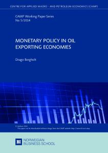
1. Monetary Policy in a Small Open Economy 1.1. Outline of the Model We construct a two-sector model of a small open economy. Two goods are produced: a non-traded good and an export good, which has a price fixed on world markets. Domestic agents consume the non-traded good and a foreign import good. The model exhibits the following three features: (a) nominal rigidities, in the form of costs of price adjustment for non-traded goods firms; (b) lending constraints on investment financing (in each sector), combined with the requirement that investment borrowing is done in foreign currency; and (c) slow pass-through of exchange rate changes into imported good prices. Nominal rigidities are introduced in order to motivate a role for monetary policy. The presence of borrowing constraints on investment is motivated by the evidence on the importance of Ôbalance sheet constraintsÕ in emerging market economies, in particular during the Mexican and Asian crises (Krugman, 1999; Eichengreen and Hausmann, 2003; Calvo, 1999). Finally, there is increasing evidence of delayed pass-through of exchange rates to consumer prices. It is well established from Engel (1999) that deviations from the law of one price are a major factor in determining real exchange rates. Nevertheless, there are significant differences across countries in the speed with which exchange rates pass-through to import and consumer prices (Choudhri and Hakura, 2003; Devereux and Yetman, 2005). Accordingly, we consider alternative speeds of adjustment of import prices to exchange rate movements. There are four sets of domestic actors in the model: consumers, firms, entrepreneurs and the monetary authority. In addition, there is a Ôrest of worldÕ sector where foreigncurrency prices of export and import goods are set, and where lending rates are determined. Figure 1 describes a flow chart of the structure of goods and assets markets in the economy. Foreign lenders write contracts with entrepreneurs for investment financing, and domestic households borrow or lend on international financial markets. Production firms in two sectors hire labour from consumers-households and entrepreneurs, rent capital from entrepreneurs and sell goods to domestic residents and foreign importers. In addition, competitive firms use capital as well as investment to Ó Royal Economic Society 2006

482

THE ECONOMIC JOURNAL

[APRIL

Monetary Authority Interest Rate Rule

Labour Supply

Goods Demand Production firms Supply of Capital Entrepreneurs Non-traded goods Export/Non-traded Export goods Wages, Profits Goods Demand

ConsumersHouseholds

Financial Contracts

Bond Trade

Labour Supply

Import Goods Demand Importers

Foreign Lenders

Unfinished Supply of Goods Capital Capital Demand Goods Unfinished Capital Goods Firms

Import Goods Demand Fig. 1.

Flow Chart for the Economy

produce Ôunfinished capital goodsÕ, which are sold to entrepreneurs. The monetary authority sets nominal interest rates. As a comparison, we will also examine a more standard economy, without financial frictions, where investment is done by domestic households. 1.2. Consumers There is a continuum of consumers/households of measure one. The representative consumer has preferences given by ! 1 1
r X Ht1þw t Ct U ¼ E0
g b ; ð1Þ 1
r 1þw t¼0 where Ct is a composite consumption index, and Ht is labour supply. Composite consumption is a CES function of consumption of non-traded goods and import goods, 1

q
1

1

q
1

where Ct ¼ a q CNtq þ ð1
aÞq CMtq , where q > 0. The implied consumer price index is 1
q 1
q then Pt ¼ aPNt þ ð1
aÞPMt , with PNt (PMt) defined as the time t price of the nontraded (import) good. Since we wish to introduce nominal price setting in the nontraded goods sector, we must allow for imperfect competition in that sector. The consumption of both non-traded and import goods is differentiated, with elasticity of substitution across i varieties equal to k, so that for non-traded goods, k hR k
1 k
1 1 CNt ¼ 0 CNt ðiÞ k di , with k > 1. Households may borrow and lend in the form of fixed-interest bonds denominated in domestic or foreign currency. Trade in foreign currency bonds is subject to small portfolio adjustment costs. If the household borrows an amount Dt, then these port 2 (denominated in the composite good), folio adjustment costs are wD =2ðDtþ1
DÞ Ó Royal Economic Society 2006

2006 ]

EXCHANGE RATES AND MONETARY POLICY

483

where D is an exogenous steady state level of net foreign debt.4 The household can borrow directly in terms of foreign currency at a given interest rate it , or in domestic currency assets at an interest rate it. The consumer credit market is not subject to informational frictions.5 Households own all home production firms and therefore receive the profits on these firms. Since export good firms and unfinished capital goods firms are perfectly competitive, profits are zero. But profits are earned by monopoly firms in the nontraded sector. A consumer’s revenue flow in any period then comes from the supply of hours of work to firms for wages Wt, transfers Tt from government, profits from the non-traded sector Pt, less debt repayment from last period ð1 þ it ÞSt Dt þ ð1 þ it ÞBt , as well as portfolio adjustment costs. Here St is the nominal exchange rate, Dt is the outstanding amount of foreign-currency debt, and Bt is the stock of domestic-currency debt. The household then obtains new loans from the domestic and/or international capital market, and uses these to consume. Her budget constraint is thus Pt Ct ¼ Wt Ht þ Tt þ Pt þ St Dtþ1 þ Btþ1 w  2
ð1 þ i  ÞSt Dt
ð1 þ it ÞBt :
Pt D ðDtþ1
DÞ t 2

ð2Þ

The household will choose non-traded and imported goods to minimise expenditure conditional on total composite demand. Demand for non-traded and imported goods is then

q PNt CNt ¼ a Ct ð3Þ Pt CMt ¼ ð1
aÞ



q PMt Ct : Pt

The household optimum can be characterised by the following conditions:     1 wD Pt Ctr Pt Stþ1  1
ðD
DÞ ¼ bE tþ1 t  r P 1 þ itþ1 St Ctþ1 tþ1 St

ð4Þ

ð5Þ


 1 Ctr Pt ¼ bEt r P 1 þ itþ1 Ctþ1 tþ1

ð6Þ

Wt ¼ gLtw Pt Ctr :

ð7Þ

4 As in Schmitt-Grohe´ and Uribe (2003), these portfolio adjustment costs eliminate the unit root in the economy’s net foreign assets. 5 We follow the majority of papers in this literature by assuming away any collateral constraints for consumer borrowing (BGG; Carlstrom and Fuerst, 1997; Gertler et al., 2001; Choi and Cook, 2004; Cook, 2004). Ce´spedes et al. (2002a,b) by contrast assume that households have to consume their current earnings, without any access to capital markets.

Ó Royal Economic Society 2006

484

THE ECONOMIC JOURNAL

[APRIL

Equations (5) and (6) represent the Euler equation for the purchase of foreign and domestic currency bonds. Equation (7) is the labour supply equation. The combination of (5) and (6) gives the representation of interest rate parity for this model. 1.3. Production Firms The two final goods sectors differ in their production technologies. Both goods are produced by combining labour and capital. As in BGG, labour comes from both households and from entrepreneurs. Thus, in the non-traded sector, effective labour of firm i is defined as e LNt ðiÞ ¼ HNt ðiÞX HNt ðiÞ1
X ;

ð8Þ

e ðiÞ is employment of where HNt(i) is employment of household labour and HNt entrepreneursÕ labour. The overall production technology for a firm in the non-traded goods sector is then

YNt ðiÞ ¼ AN KNt ðiÞa LNt ðiÞ1
a ;

ð9Þ

where AN is a productivity parameter. Exporters (all domestically-produced traded goods are exported) use the production function YXt ðiÞ ¼ AX KXt ðiÞa LXt ðiÞ1
a :

ð10Þ

Final goods firms in each sector hire labour and capital from consumers and entrepreneurs, and sell their output to consumers, entrepreneurs (for their consumption) and capital-producing firms. Cost minimising behaviour then implies the following equations:

Wt ¼ MCNt ð1
aÞX

YNt HNt

WNte ¼ MCNt ð1
aÞð1
XÞ

RNt ¼ MCNt a

YNt e HNt

YNt KNt

Wt ¼ PXt ð1
cÞX

ð12Þ

ð13Þ

YXt HXt

WXte ¼ PXt ð1
cÞð1
XÞ Ó Royal Economic Society 2006

ð11Þ

ð14Þ

YXt e HXt

ð15Þ

2006 ]

EXCHANGE RATES AND MONETARY POLICY

RXt ¼ PXt c

YXt : KXt

485 ð16Þ

Equations (11)–(13) describe the choice of employment of households and entrepreneurs and demand for capital which achieves cost minimisation in the non-traded goods sector, where MCNt denotes the marginal cost in that sector. Equations (14)–(16) characterise cost minimisation in the export good sector. Note that the price of the traded export good is PXt. Since the export sector is competitive, PXt represents the unit cost of production. Movements in this price, relative to the import price PMt, represent terms of trade fluctuations for the small economy. There are adjustment costs of investment, so that the marginal return to investment in terms of capital goods is declining in the amount of investment undertaken, relative to the current capital stock. Capital stocks in the non-traded and export sectors evolve according to "
2 # INt /D INt KNtþ1 ¼

d ð17Þ KNt þ ð1
dÞKNt KNt 2 KNt  KXtþ1 ¼


 IXt /D IXt

d2 KXt þ ð1
dÞKXt : KXt 2 KXt

ð18Þ

Investment in new capital requires imports and non-traded goods in the same mix as the household’s consumption basket. Thus, the nominal price of a unit of investment, in either sector, is Pt. As described in Figure 1, competitive firms produce unfinished capital goods and sell them to entrepreneurs. We may think of these firms as combining investment (in the same composite as domestic consumption) and the existing capital stock to produce new capital goods using the production functions implicit in (17) and (18). For instance, in the non-traded sector, competitive capital-producing firms will ensure that the price of capital sold to entrepreneurs is QNt ¼

Pt : 1
/D ðINt =KNt
dÞ

ð19Þ

This gives an implicit investment demand in each sector, depending on the sector specific ÔTobin’s qÕ.6 1.4. Price Setting Firms in the non-traded sector set their prices as monopolistic competitors. We follow Rotemberg (1982) in assuming that each firm bears a small direct cost of price 6 For example, in the non-traded sector, new capital is produced using the production function G(IN, KN) ¼ (IN/KN
/D/2(IN/KN
d)2]KN, and unfinished capital goods firms maximise profits, given by G G KN , where RKN is the rental rate on non-tradeable capital in the unfinished goods QN GðIN ; KN Þ
PIN
RKN capital sector – see the Appendix for details. Note that, if there were no adjustment costs of accumulation, then capital-producing firms would simply use final goods investment alone, and Q ¼ P would hold.

Ó Royal Economic Society 2006

486

THE ECONOMIC JOURNAL

[APRIL

adjustment. As a result, firms will only adjust prices gradually in response to a shock to demand or marginal cost. Non-traded firms are owned by domestic households. Thus, a firm will maximise its expected profit stream, using the households discount factor. We define the discount factor as follows Ct ¼

br : Pt Ctr

Using this, we may define the objective function of the non-tradable firm i as: (   ) 1 X wPN PNt ðiÞ
PNt
1 ðiÞ 2 E0 Ct PNt ðiÞYNt ðiÞ
MCNt YNt ðiÞ
Pt ; PNt ðiÞ 2 t¼0

ð20Þ

ð21Þ

where C0 ¼ 1, YNt(i) ¼ [PNt(i)/PNt]
kYNt represents total demand for firm iÕs nontraded product, and the third expression inside parentheses describes the cost of price change that is incurred by the firm. Firm i chooses its price to maximise (21). Since all non-traded goods firms are alike, after imposing symmetry, we may write the optimal price setting equation as:
 wPN Pt PNt k PNt PNt ¼ MCNt

1 k
1 k
1 YNt PNt
1 PNt
1 
 ð22Þ wPN Ctþ1 Ptþ1 PNtþ1 PNtþ1 þ Et
1 : k
1 Ct YNt PNt PNt When the parameter wPN is zero, firms simply set price as a markup over marginal cost. In general, however, the non-traded goods price follows a dynamic adjustment process.

1.5. Local Currency Pricing We assume that the law of one price must hold for export goods, so that  PXt ¼ St PXt :

ð23Þ

For import goods however, we allow for the possibility that there is some delay between movements in the exchange rate and the adjustment of imported goods prices. The assumption is that there is a set of monopolistic domestic importers (owned by home households) who purchase the foreign good at prices St PMt and then sell to the home market at PMt. These importers face cost of price adjustment of the same faced by nontraded firms. Thus, the imported good price index for domestic consumers moves as
 w k Pt PMt PMt  PMt ¼ St PMt
PM
1 k
1 k
1 TMt PMt
1 PMt
1 
 ð24Þ wPM Ctþ1 Ptþ1 PMtþ1 PMtþ1 þ Et
1 : k
1 Ct TMt PMt PMt The interpretation of (24) is that the monopolistic competitive firm wishes to see the domestic price as a markup over the foreign price. But it incurs quadratic price adjustment costs, and unless wPM ¼ 0, it will move its price only gradually towards the Ó Royal Economic Society 2006

2006 ]

EXCHANGE RATES AND MONETARY POLICY

487

desired price. The higher are these adjustment costs, the lower will be the rate of exchange rate pass-through into imported goods prices facing the domestic consumer.7 1.6. Entrepreneurs Unfinished capital is transformed by entrepreneurs and sold to the final goods sector. But entrepreneurs must borrow in order to finance their investment. In modelling the actions of entrepreneurs we follow the set-up of BGG, extending their closed-economy model of investment financing to the two-sector open economy. The details of the entrepreneurial sector and calibration of the external risk premium are set out fully in the Appendix. Here we give an intuitive account of the process. Entrepreneurs borrow from foreign lenders, in order to finance their investment projects, which produce finished capital goods. But each project exhibits idiosyncratic productivity x 2 (0, 1), drawn from a distribution F(x), with pdf f(x), and E(x) ¼ 1. Productivity x is observed by the entrepreneur but can only be observed by the lender through costly monitoring. The borrowing arrangement between lenders and entrepreneurs is then constrained by the presence of private information. The optimal contract is a debt contract, which specifies a given amount of lending, and a state If the entrepreneur redependent threshold level of entrepreneurial productivity x.  times the return on ports productivity exceeding the threshold, then a fixed payment x capital is made to the lender and no monitoring takes place. But if reported productivity falls short of the threshold, then the lender monitors, incurring a monitoring cost l times the value of the project and receives the full residual amount of the project. The effect of this lending contract is to make borrowing more costly for entrepreneurs than financing investment out of internal resources. Moreover, the borrowing premium depends on the entrepreneur’s net worth, relative to the total borrowing requirement. There are two groups of entrepreneurs, one in each sector of the economy. Entrepreneurs borrow in foreign currency by assumption.8 An entrepreneur j in the nonj j tradable sector wishing to invest KNtþ1 units of capital must pay nominal price KNtþ1 QNt to the unfinished capital good firm. Say that the entrepreneur begins with nominal net worth in domestic currency given by ZNtþ1 . Then she must borrow in foreign currency an amount given by e;j

Dtþ1 ¼

1 j j ðQNt KNtþ1
ZNtþ1 Þ: St

ð25Þ

The total expected return on the investment is Et(RKNtþ1QNtKNtþ1) (where RKNtþ1 is defined below).  Ntþ1 , The optimal contract stipulates a cut-off value of the firm’s productivity draw, x and an investment level, KNtþ1. Under this contract structure, the entrepreneur receives 7 Note that the import firm faces elasticity k also, as we have assumed that the elasticity of substitution across types of imports is the same as that across types of non-traded goods. TMt is the total demand for imports of the domestic country. 8 Eichengreen and Hausmann (2003) provide ample evidence that borrowing in foreign currency is a constraint on most emerging economies. The reason for this constraint is a subject of ongoing research. See for instance Schneider and Tornell (2004).

Ó Royal Economic Society 2006

488

THE ECONOMIC JOURNAL

[APRIL

 Ntþ1 Þ, of the total return, and the lender receives share Bðx  Ntþ1 Þ. an expected share Aðx  Ntþ1 Þ þ Bðx  Ntþ1 Þ ¼ 1
/Ntþ1 , where /Ntþ1 represents the expected cost of In sum, Aðx monitoring.9 As shown in the Appendix, the first order conditions for the optimal contract can be arranged to obtain the following two equations:  Ntþ1 ÞA0 ðx  Ntþ1 Þ=B 0 ðx  Ntþ1 Þ
Aðx  Ntþ1 Þg Et fRKNtþ1 ½Bðx  ¼ ð1 þ itþ1 Þ  Ntþ1 Þ=½B 0 ðx  Ntþ1 ÞStþ1 =St g Et fA0 ðx

ð26Þ


 RKNtþ1 St ZNtþ1   Ntþ1 Þ ¼ ð1 þ itþ1 Bðx Þ 1
: Stþ1 QNt KNtþ1

ð27Þ

Equation (26) represents the relationship between the expected return on entrepreneurial investment in the non-traded sector and the opportunity cost of investment. In the absence of private information (or with zero monitoring costs), the expected return would equal the opportunity cost of funds for the lender. But in general, the presence of moral hazard in the lending environment imposes an external finance  premium, so that EðRKNtþ1 Þ  ð1 þ itþ1 ÞEðStþ1 =St Þ. The extent of this premium  N . The key feature of the BGG framework is that this depends on the value of x premium is linked to the amount borrowed. This relationship is seen in (27), which represents the participation constraint for the lender. The smaller is the entrepreneur’s net worth ZNtþ1 relative to investment QNtKNtþ1, the more the entrepreneur must borrow. Equations (26) and (27) may then be used (see the Appendix of BGG) to show  that the external finance premium EðRKNtþ1 Þ=½ð1 þ itþ1 ÞEðStþ1 =St Þ is increasing in the leverage ratio QNtKNtþ1/ZNtþ1. A fall in entrepreneurial net worth (for instance, generated by a nominal exchange rate depreciation), will directly reduce investment, by raising the external finance premium, and increasing the cost of capital to the entrepreneur. This captures the Ôfinancial acceleratorÕ mechanism discussed by BGG. How is entrepreneurial net worth determined? As in Carlstrom and Fuerst (1997) and BGG, the entrepreneurial sector must be designed so that entrepreneurs are always constrained by the need to borrow. The simplest way to allow for this is to assume that a new infusion of entrepreneurs arrives in every period and a fraction of the existing stock of entrepreneurs randomly die, keeping the total population constant. In this way, entrepreneurs do not build up wealth to the extent that the borrowing constraint is non-binding. At the beginning of each period, a non-defaulting entrepreneur j in the non-traded  Nt . Entrepreneurs sector receives the return on investment RkNt QNt
1 KNt ðjÞ½xNt ðjÞ
x die at any time period with probability (1
m). They consume only in the period in which they die. Thus, at any given period, a fraction (1
m) of the return on capital to entrepreneurs is consumed. Because entrepreneurial risk is i.i.d., the functional forms used here allow for aggregation, so that the mean return on capital in each sector is

R R 9   and /RN may be written Ras follows; AðxÞ  ¼ x1 xf ðxÞdx
x  x1 f ðxÞdx, BðxÞ  ¼ BðxÞ R 1Aðx),   x x  x f ðxÞdx þ ð1
lÞ 0 xf ðxÞdx, /N ¼ l 0 xf ðxÞdx. It is straightforward to show that A0 ðxÞ   0, and x 0  B ðxÞ  0. Ó Royal Economic Society 2006

2006 ]

EXCHANGE RATES AND MONETARY POLICY

489

 Nt Þ. Aggregate net worth is then determined by the unconsumed RkNt QNt
1 KNt Aðx fraction of the return on capital, as well as wages earned by entrepreneurs working in the non-tradable sector. Thus,  Nt Þ þ WNte : ZNtþ1 ¼ mRKNt QNt
1 KNt Aðx

ð28Þ

 and the lender’s participation constraint, we may rewrite Using the definition of AðxÞ this as ZNtþ1 ¼ mð1
/Nt ÞRKNt QNt
1 KNt
mð1 þ it ÞðSt =St
1 ÞðQNt
1 KNt
ZNt Þ þ WNte :

ð29Þ

Note that net worth depends negatively on the current exchange rate, since an unanticipated increase in the exchange rate raises the value of existing foreign currency liabilities for the firm. This adds a non-traditional mechanism for the evaluation of alternative exchange rate rules. The details of the contract structure and net worth dynamics in the export sector are described in the identical way. Finally, we may define the return to capital for entrepreneurs. Entrepreneurs rent their finished capital to both final-goods firms and also to firms who produce unfinished capital goods through investment and the use of existing capital (the production function for this is implicit in the adjustment cost technologies (17) and (18)). The real return on capital is then written as the sum of the nominal rental rate on capital earned from final-goods production firms, the rental rate earned from the firms producing unfinished capital goods firms, plus the value of the non-depreciated capital stock, divided by the original price of capital. Thus we write the rate of return as
     1 INtþ1 INtþ1 wI INtþ1 RKNtþ1 ¼ RNtþ1 þ 1
d þ wI
d
ð
dÞ2 QNtþ1 : ð30Þ QNt KNtþ1 KNtþ1 2 KNtþ1 1.7. Monetary Policy Rules The monetary authority uses a short-term interest rate as the monetary instrument. The general form of the interest rate rule used may be written as )l p

 ( PNt 1 lpn Pt 1 S t lS  ð31Þ 1 þ itþ1 ¼ ð1 þ iÞ: 1 n  PNt
1 p S ½aðPNt
1 Þ1
q þ ð1
aÞðPMt
1 Þ1
q 1
q p The parameter lpn allows the monetary authority to control the inflation rate in the non-traded goods sector around a target rate of pn . The parameter lp governs the degree to which the CPI inflation rate is targeted at the desired level of p. Finally, lS controls the degree to which interest rates attempt to control variations in the ex We compare the properties of alternative change rate, around a target level of S. exchange rate regimes under a variety of different assumptions regarding the values of these policy coefficients.10

10

In each case, we set policy so that the equilibrium is determinate.

Ó Royal Economic Society 2006

490

THE ECONOMIC JOURNAL

[APRIL

1.8. Equilibrium In each period, the non-traded goods market must clear. Thus, we have

q  PNt w 2 YNt ¼ a Ct þ INt þ IXt þ CtNe þ CtXe þ D ðDtþ1
DÞ Pt 2 !2 3
2 wPN wPM PMT PNt GNt KNt GXt KXt þ
1 þ /Nt þ /Xt þ
1 5: 2 PNt
1 Pt Pt 2 PMTt
1

ð32Þ

where GNt ¼ RkNt QNt
1 Equation (32) indicates that demand for non-traded goods comes from household consumption, investment and the consumption of entrepreneurs. In addition, because portfolio adjustment costs, costs of price adjustment and the costs of monitoring loans in each sector are represented in terms of the composite final good, part of these costs must be incurred in terms of non-traded goods. The demand for the import good TMt can be derived analogously (see Appendix). The aggregate balance of payments condition for the economy may be derived by adding the budget constraint of the household and the entrepreneurs in each sector. We may write it as wD  2 þ St ð1 þ i  ÞðDt þ D e Þ ðDtþ1
DÞ t t 2 2 wP ðPNt
PNt
1 Þ þ Pt N þ ð/Nt RkNt KNt QNt
1 þ /Xt RkXt KXt QXt
1 Þ 2 2 PNt
1

e e Pt Ct þ Pt CNt þ Pt CXt þ Pt

ð33Þ

e þ Pt ðINt þ IXt Þ ¼ PNt YNt þ PXt YXt þ St ðDtþ1 þ Dtþ1 Þ þ PMt :

This just says that total expenditures, which comprise of consumption of households, entrepreneurs in each sector, investment in each sector, bond adjustment costs, price adjustment costs, monitoring costs, and total foreign debt repayment (the sum of private and entrepreneurial debt), must equal total receipts, which are output of each sector, plus new net foreign borrowing, plus the profits from the import sector, PMt. In addition, both the households and the entrepreneur labour market conditions must be satisfied: HXt þ HNt ¼ Lt

ð34Þ

e ¼1 HXt

ð35Þ

e ¼ 1: HNt

ð36Þ

1.9. Comparison Economy Without Entrepreneurs In order to explore the importance of financing constraints, we also solve the model under the more conventional assumptions about the financing of capital accumulation.

Ó Royal Economic Society 2006

2006 ]

EXCHANGE RATES AND MONETARY POLICY

491

In this economy, investment is done directly by households, and there are no entrepreneurs or external finance premium on investment.11 This alters only the equations governing the household budget constraint and the Euler equation for the determination of sectoral capital. The Appendix outlines this economy in detail.

2. Calibration and Solution We now derive a numerical solution for the model, by first calibrating and then simulating. The calibration of the model is somewhat more complicated than the usual dynamic general equilibrium framework, since the model has two production sectors and it involves parameters describing the entrepreneurial sector. The benchmark parameter choices for the model are described in Table 1. Some standard parameter values are those governing preferences. It is assumed that the intertemporal elasticity of substitution in consumption is 0.5. This is within the range of the literature. Following Stockman and Tesar (1995), we set the elasticity of substitution between non-traded and imported goods in consumption to unity.12 The elasticity of labour supply is also set to unity, following Christiano et al. (1997). In addition, the elasticity of substitution between varieties of non-tradable goods determines the average price–cost mark-up in the non-tradable sector. We follow standard estimates from the literature in setting a 10% mark-up, so that k ¼ 11 (an identical value is assumed for the elasticity of substitution between varieties of imports). Assuming that the small economy starts out in a steady state with zero consumption growth, the world interest rate must equal the rate of time preference. We set the world Table 1 Calibration of the Model Parameter r b q k g w c a d a wPN wI wD rx l m X

Value

Description

2 0.985 1

Inverse of elasticity of substitution in consumption Discount factor (quarterly real interest rate is (1
b)/b) Elasticity of substitution between non-traded goods and import goods in consumption Elasticity of substitution between varieties (same across sectors) Coefficient on labour in utility Elasticity of labour supply Share of capital in export sector Share of capital in non-traded sector Quarterly rate of capital depreciation (same across sectors) Share on non-traded goods in CPI Price adjustment cost in the non-traded sector Investment adjustment cost (same across sectors) Bond adjustment cost Standard error of the technology shock of entrepreneurs Coefficient of monitoring cost for lenders Aggregate saving rate of entrepreneurs Share of householdsÕ labour in the effective labour

11 1.0 1.0 0.7 0.3 0.025 0.55 120 12 0.0007 0.5 0.2 0.94 0.95

11 The dynamics of this economy are effectively identical to one where there are entrepreneurs that finance investment but information on their returns is public. Focusing on a model without entrepreneurs makes our results more comparable with previous literature. 12 Mendoza (1995) uses a smaller value of 0.67. Using the lower value would not affect our results.

Ó Royal Economic Society 2006

492

THE ECONOMIC JOURNAL

[APRIL

interest rate equal to 6% annually, an approximate number used in the macro-RBC literature, so that at the quarterly level, this implies a value of 0.985 for the discount factor. We set D so that steady state debt is 40% of GDP, approximately that for East Asian economies in the late 1990s. The factor intensity parameters are quite important in determining the dynamics of the model. In the short run, only labour is mobile between sectors, so the impact of interest rate and terms of trade shocks on output will depend on the labour intensity of the different sectors. For two Asian economies, Malaysia and Thailand, Cook and Devereux (2001) find that the non-traded sector is more labour intensive than the traded sector. Both country’s estimates of sectoral wage shares are quite similar. Following these estimates, we set total share of labour in GDP to 52%, the labour share of traded goods (i.e. export) output to 30%, and the share of wages in non-traded output to 70%. In combination with the other parameters of the model, the parameter a, governing the share of non-traded goods in the CPI, determines the share of nontraded goods in GDP. Following the classification followed by De Gregorio et al. (1994), we found that the average share of non-traded goods in total GDP in Thailand was 54% over the period 1980–98. Cook and Devereux (2001) find a similar figure for Malaysia. Given the other parameters, this implies a value of a equal to 0.55. We follow BGG in setting /I so that the elasticity of Tobin’s q with respect to the investment capital ratio is 0.3. With respect to the costs of portfolio adjustment, we follow the estimate of Schmitt-Grohe´ and Uribe (2003) to set wD ¼ 0.0007. To determine the degree of nominal rigidity in the model, we set the parameter governing the cost of price adjustment, /PN so that, if the model were interpreted as being governed by the dynamics of the standard Calvo price adjustment process, all prices would adjust on average after 4 quarters. This follows the standard estimate used in the literature (Chari et al., 2000). To match this degree of price adjustment requires a value of /PN ¼ 120. We consider two values for the import price pass-through variable, setting /PM ¼ 0 and /PM ¼ 120. The former represents the complete pass-through case; the latter implies the same degree of price stickiness in the import sector as governs the non-tradable good sector. We follow BGG in choosing a steady-state risk spread of 200 basis points. We set a leverage ratio of 3, higher than BGG (who use 2), but more consistent with the higher leverage observed in emerging market countries. In addition, we assume a bankruptcy cost parameter l equal to 0.2, roughly mid-way between that of Carlstrom and Fuerst (1997) and BGG. Finally, given the other parameters chosen, the implied savings rate of entrepreneurs is 0.94. We consider two types of external shock: (a) shocks to the world interest rate; and (b) terms of trade shocks. In the model, (a) is represented by shocks to it ; and (b) is represented by shocks to

PX =PM .

The general form of the interest rule (31) allows for a variety of different types of monetary policy stances. We focus the investigation by limiting our analysis to three types of rules. The first rule is one whereby the monetary authorities target the inflation rate of non-traded goods prices (NTP rule), so that lpn ! 1. This is analogous to the targeting Ó Royal Economic Society 2006

2006 ]

EXCHANGE RATES AND MONETARY POLICY

493

of domestic inflation that is analysed in a number of recent papers (Benigno, 2001). The general rationale for such a rule is that by adjusting the monetary instrument to prevent inflation in non-traded goods, it eliminates the need for non-traded goods producers to adjust their prices, so that their inability to change prices quickly becomes irrelevant. In the absence of other nominal rigidities or distortions, this policy would replicate the real response of the flexible price economy. We also analyse a CPI targeting rule (CPI rule), whereby the monetary authority targets the domestic consumer price index lp ! 1. This is motivated by the fact that the CPI is the most common index used in practice by those countries that follow a policy of explicit inflation targeting. With high exchange rate pass-through, the price stability rule is very similar to an exchange rate peg, while with delayed pass-through, it is closer to the non-traded goods price targeting. Finally, we analyse a simple fixed exchange rate lS ! 1, whereby the monetary authorities adjust interest rates so as to keep the nominal exchange rate from changing. The model is solved numerically using a second order approximation to the true dynamic stochastic system, where the approximation is done around the non-stochastic steady state. It is necessary to use a second order approximation because we wish to compare alternative monetary rules in terms of welfare, where welfare is represented by the expected utility of households and entrepreneurs. As discussed by Woodford (2003) and Schmitt-Grohe´ and Uribe (2004a), a second-order-accurate representation of expected utility can be obtained only through a second-order representation of the underlying dynamic system, except in special cases. Hence, to evaluate expected utility, we use the method of Schmitt-Grohe´ and Uribe (2004a) in computing a second-order representation of the model.13

3. External Shocks under Alternative Monetary Rules Here we explore the impact of shocks under the three alternative monetary rules. In order to illustrate the workings of the model, we assume that both shocks may be described as AR(1) processes with persistence 0.46 and 0.77, for the interest rate and terms of trade shock respectively. This corresponds quite closely to our empirical estimates for Asia, discussed below. The Figures show alternatively how the collateral constraints and the speed of exchange rate pass-through determine the transmission of shocks to the economy. The illustrations are divided into categories of real variables (namely, total output; employment; the trade balance; absorption; the real exchange rate; the real interest rate; and sectoral outputs) and those of nominal or financial variables (namely, overall inflation; the nominal exchange rate; the nominal interest rate; and the inflation rate for imported goods). 3.1. Interest Rate Shocks Figures 2–4 illustrate the effect of a persistent shock to the world interest rate. Figures 2 and 3 show the impact of the shock without and with the presence of financing 13 Our solution is obtained using Schmitt-Grohe´ and Uribe’s MATLAB code, available at http://www. econ.upenn.edu/uribe/2ndorder.htm

Ó Royal Economic Society 2006

494

[APRIL

THE ECONOMIC JOURNAL Output to i*

Employment to i*

Trade Balance to i*

0.02

0.05

0.6

0

0

0.4

NPT Fix E CPI −0.02

−0.05

0.2

NPT

NPT

Fix E

−0.04

Fix E

−0.1

CPI

0

CPI

−0.06

−0.15 0

10

20

−0.2 0

Absorption to i*

10

20

0

Real EX to i*

0

0.2

−0.1

0.15

20

10 NPT

NPT

Fix E

Fix E 5

CPI −0.2

10 Real i to i*

CPI

0.1 NPT

0

Fix E

−0.3

0.05

CPI −0.4

0 0

10 NT Output to

−5

20

0

i*

10 Traded Output to

0.1

0.3

0

0.2

20

0

i*

Inflation to

20 i*

0.3 NPT

NPT

Fix E

0.2

Fix E

CPI

CPI −0.1

10

0.1

0.1

0

0

NPT Fix E

−0.2

CPI −0.3 0

10

20

−0.1 0

Nominal EX to i*

−0.1 10 Nominal i to i*

0.3

10

0.2

0

20

20

0.6

NPT

NPT

Fix E

Fix E 5

CPI

10 Traded Good π to i* NPT Fix E

0.4

CPI

CPI

0.1

0.2 0

0

0

−0.1

−5 0

10

Fig. 2.

20

−0.2 0

10

20

0

10

Impulse Response to i : No Financial Constraint, Full Pass-through

Ó Royal Economic Society 2006

20

2006 ]

EXCHANGE RATES AND MONETARY POLICY

495

constraints respectively, under complete pass-through in import prices (i.e. assuming that /PM ¼ 0). The unanticipated rise in the cost of external borrowing leads first to a fall in total absorption, so that both private consumption and investment fall. The fall in absorption causes a fall in demand for non-traded goods, leading to a real exchange rate depreciation. Non-traded output falls, while output in the export sector will rise, and the economy experiences an increase in the trade surplus. In principle, the impact of the interest rate spike on output is ambiguous, since total output is a combination of non-traded and export sector output. As Figure 2 shows, the output impact of the interest rate shock depends critically on the monetary rule. The NTP rule involves an expansionary monetary policy, since the fall in demand tends to generate a deflation in the non-traded goods sector and, in order to prevent the pressure for non-traded goods prices to fall, monetary policy must be expansionary. The NTP rule in this case in fact sustains the flexible-price response of the economy. Aggregate output and employment expand slightly under this rule. Note also however that the NTP rule requires a very large nominal exchange rate depreciation, followed by an appreciation. Due to high exchange rate pass-through, this means a large initial burst of inflation. The mechanism by which this stabilises GDP is seen in Figure 2. The immediate but temporary rise in the nominal exchange rate leads to a cushioning of the nominal and real interest rate from the full effects of the rise in foreign borrowing. The domestic real interest rate rises by less than half of the rise in the foreign interest rate. This is because at the date of the shock, the real exchange rate is expected to appreciate, following the initial large depreciation. Since the real interest rate for domestic households is monotonically related to the anticipated real exchange rate depreciation, the expected real appreciation reduces the overall increase in the real interest rate, and cushions the impact of the shock on absorption, demand, and GDP. Under the other two policy rules, however, the interest rate shock tends to be highly contractionary. Moreover, the exchange rate peg and the inflation target have almost the same implications. Both rules must act so as to prevent a nominal exchange rate depreciation: the fixed exchange rate rule does this by design, while the CPI rule must essentially stabilise the exchange rate in order to stabilise the CPI in face of sticky nontraded goods prices. By preventing an immediate real exchange rate depreciation, these policies prevent the cushioning of the shock on the real interest rate and ensure that the full impact of the foreign real interest rate shock is passed through to the domestic economy. There is a much larger fall in absorption, output in the non-traded sector and overall GDP. Now we see that total employment falls. On the other hand, the lower level of total absorption implies a larger trade surplus. How does the presence of a collateral constraint in investment financing affect this conclusion? Figure 3 illustrates the impact of the same foreign interest rate shock in the model with entrepreneurs and investment financing constraints. The key effect of the financing constraints is to increase the downward shift of investment and, so, overall absorption. This occurs because the higher borrowing costs reduce the value of existing capital for entrepreneurs in each sector, and also because the unanticipated real exchange rate depreciation raises the debt burden for entrepreneurs. Both channels reduce net worth, raising the effective cost of borrowing and reducing Ó Royal Economic Society 2006

496 Output to i*

Employment to i*

0.05

0.1

0

0

NPT Fix E CPI

−0.1

0

10 Real EX to i*

20

−0.3

0.3

0.5

0

10 Real i to i*

20

5

0.1

10 Inflation to i*

20

0.3

−5

0.2

0

10 20 NT Output to i*

0

10 20 Nominal EX to i*

0.3

−0.2

0.2

0.6

−0.8

0

10 Nominal i to i*

20

−0.1

10

0.2

0

0.2

0

0

Fig. 3.

20

0

0

10

20

−5

NPT Fix E CPI

0

10 20 Traded Good π to i*

0

10

NPT Fix E CPI

0.4

5

10

10 20 Traded Output to i*

0.6 NPT Fix E CPI

0.4

0

0

0

0.1

−0.1

NPT Fix E CPI

0.1 NPT Fix E CPI

15 NPT Fix E CPI

−0.8

0

−0.6

0.8 NPT Fix E CPI

0

−0.4

0

0

−0.4 −0.6

NPT Fix E CPI

10

0.2

−0.2

NPT Fix E CPI

15 NPT Fix E CPI

Absorption to i* 0

NPT Fix E CPI

−0.2

0.4

0

Trade balance to i* 1

−0.1

−0.05

−0.15

[APRIL

THE ECONOMIC JOURNAL

20

−0.2

0

10

20

Impulse Response to i : With Financial Constraint, Full Pass-through

investment by more than we see in the model without financing constraints. In the aggregate, it follows that the impact of the financing constraints is to magnify the impact of the interest rate shock. Output and employment fall by more, and the trade balance increases by more, since the greater fall in absorption causes a sharper collapse in non-traded output, and traded goods output rises by more than the economy without financing constraints. In this economy, the role of financing constraints is to increase the ÔmultiplierÕ effect of external shocks significantly. But from the figures, it is clear that the financing constraints have essentially no effect on the rankings of the alternative policy rules. The NTP rule still acts so as to cushion output from the interest shock. But the fixed exchange rate and CPI rule lead to much greater responses in real variables than the NTP rule. Hence, the ranking of alternative policies remains the same as in the economy without financing constraints. Just as the impact of financing constraints is to increase the response of real aggregates, it also implies a magnified response of exchange rates and prices. The NTP rule requires a much higher response of the nominal and real exchange in the presence of financing constraints. As a result, the inflationary consequences of the NTP rule are significantly greater in the presence of financing constraints: the initial jump in Ó Royal Economic Society 2006

2006 ] Output to i*

Employment to i*

0.1 NPT Fix E CPI

0.05 0

Trade Balance to i*

0.2

0.6

0.1

0.4

0

−0.05 −0.1

NPT Fix E CPI

−0.1

0

10 Real EX to i*

20

0.4

−0.2

0

10 Real i to i*

20

10 NPT Fix E CPI

0.3

NPT Fix E CPI

5

0.2

0

10 Inflation to i*

20

0.02

NPT Fix E CPI

−0.1

0.2

−0.2

0

−0.3

−0.2

0

10 NT Output to i*

20

−5

0

10 20 Nominal EX to i*

0.3

0

0.2

0.2

−0.02

−0.3

−0.04

0

10

0

10 Nominal i to i*

20

Fig. 4.

−0.1

10 20 Traded Output to i* NPT Fix E CPI

−0.1

0

10 20 Traded Good π to i*

0.06 NPT Fix E CPI

5

0.04

NPT Fix E CPI

0.02 0

0

20

0

0

0.1 NPT Fix E CPI

NPT Fix E CPI

0.1 NPT Fix E CPI

10 NPT Fix E CPI

−0.4

0.1

−0.2

0.3

0

−0.06

Absorption to i* 0

−0.1 0

0.1 0

497

EXCHANGE RATES AND MONETARY POLICY

0

10

20

−5

0

0

10

20

−0.02 0

10

20

Impulse Response to i : No Financial Constraint, Delayed Pass-through

both the exchange rate and the consumer price level after an interest rate shock is almost twice that of the economy without financing constraints. The results so far are based on the assumption that exchange rate pass-through to imported goods prices is immediate. How does the presence of delayed pass-through affect the results? We now let /PM ¼ 120, so that price adjustment of the imported good follows the same process as that of the non-tradable good. Figure 4 illustrates the response of the economy to an interest rate shock under delayed pass-through. Note that the response under the fixed exchange rate does not change, since with a fixed exchange rate the speed of import price response to exchange rate shocks is irrelevant. From a qualitative point of view, the slower exchange rate pass-through does not change the way in which the economy responds to interest rate shocks. It is still the case that absorption falls, the trade balance improves as resources are shifted into the export sector, aggregate output falls and there is a real exchange rate depreciation. This indicates that closing off the Ôexpenditure-switchingÕ effect, by which exchange rate changes immediately affect the relative price of home to foreign goods, does not alter the qualitative dynamics of the economy. Quantitatively, however, the presence of delayed pass-through has a big effect on the response to an interest rate shock. Moreover, it has important implications for the comparison of alternative monetary policy rules. The most significant feature of Ó Royal Economic Society 2006

498

THE ECONOMIC JOURNAL

[APRIL

Figure 4, when compared with Figure 2, is that there is now a distinct difference between the performance of the CPI rule and a fixed exchange rate. When passthrough is instantaneous, a policy maker cannot stabilise CPI inflation without largely stabilising the exchange rate. But with delayed pass-through, this becomes possible. Under the CPI rule, there is a big initial depreciation in the nominal exchange rate, far larger than the exchange rate response when the same rule is applied under full passthrough. The result is that there is a substantial real depreciation, which allows the policy-maker to cushion the impact of the shock on the real interest rate. As a result, under a CPI rule, the fall in total absorption and GDP, and the rise in the trade balance is much less than in the case of immediate pass-through. The absence of pass-through therefore rationalises the use of strict inflation targeting in an emerging market, at least for dealing with shocks to the foreign interest rate. CPI targeting becomes much closer to the NTP policy rule. The NTP rule, as before, acts so as to stabilise output, by generating substantial movements in the real exchange rate. Both policy rules (NTP and CPI) operate by actively employing the nominal exchange rate in order to stabilise the effective real interest rate. It is interesting to note here that while the strict Ôexpenditure-switchingÕ mechanism for the exchange rate is greatly diminished when there is delayed exchange rate pass-through (since nominal exchange rate changes no longer alter relative prices facing consumers and firms) there is still a critical role played by the exchange rate in controlling effective real interest rates. By altering the rate of expected real exchange rate depreciation, monetary policy stabilises the economy, even in the absence of pass-through.14 A corollary of these results is that the inflation output volatility trade-off is altered by the presence of delayed pass-through. With full pass-through, the policy of stabilising non-traded goods inflation cushions the impact of an interest rate shock on GDP. But this can only be done by allowing a large initial burst of inflation, following up the exchange rate depreciation. A fixed exchange rate, on the other hand, stabilises inflation, but destabilises GDP. Hence, the trade-off between fixed and flexible exchange rates (under an NTP rule) can be described as a trade-off between output volatility and inflation volatility. But Figure 4 now shows us that both GDP and inflation can be substantially stabilised simultaneously, using either a CPI rule or an NTP rule. Indeed, we see from the Figure that the response of inflation under a fixed exchange rate is now in absolute terms as great as that under the non-traded inflation target rule. Thus, under delayed pass-through, fixing the exchange rate no longer ensures lower inflation volatility. 3.2 Terms of Trade Shocks Figures 5–7 illustrate the effect of a persistent negative shock to the terms of trade. In this model, a terms of trade shock is equivalent to a negative income shock coming from the export sector. This negative wealth effect leads to a decline in consumption and a rise in labour supply. Since it is also equivalent to a negative productivity shock in 14 An alternative perspective is to note that while the law of one price relationship no longer holds instantaneously, the interest rate parity relationship is still an important macroeconomic linkage.

Ó Royal Economic Society 2006

2006 ] Output to −TOT

Employment to −TOT

0.5

Trade Balance to −TOT 0.5

0.2 0.1

0

−1

0

0 NPT Fix E CPI

−0.1

10 20 Real EX to −TOT

−0.2 0

0.4

10 Real i to −TOT

0.3

20

10 20 Inflation to −TOT

0.2

−2

0 10 20 Nominal EX to −TOT

0.8 NPT Fix E CPI

0.1

0.4

−0.1

0.2

0

10

Fig. 5.

20

0

10 20 NT Output to −TOT

−0.5

0

−1

−0.1

10

0

10 20 Nominal i to −TOT

2

20

−2

0 10 20 Traded Output to −TOT

0

0.1

NPT Fix E CPI

0

0

−0.2 0.5

NPT Fix E CPI

4 NPT Fix E CPI

0.6

0

−0.2

NPT Fix E CPI

0

0

0

0.2

0.2

0

−1

NPT Fix E CPI

−0.1

0.3

2

0.1

NPT Fix E CPI

−0.5

4 NPT Fix E CPI

Absorption to −TOT 0.2 0.1

0

0 NPT Fix E CPI

−0.5

499

EXCHANGE RATES AND MONETARY POLICY

0

10

NPT Fix E CPI

−1.5

0 10 20 Traded Good π to −TOT 0.6 NPT 0.4 Fix E CPI 0.2 0

20

−0.2

0

10

20

Impulse Response to
TOT: No Financial Constraint, Full Pass-through

the export sector, output and employment fall in that sector. Because the shock is transitory, the trade balance deteriorates. The implications for other aggregates depend on the policy being followed. Under the NTP policy, there is a fall in the nominal interest rate, which stimulates output in the non-traded goods sector. Under the other rules, interest rates rise, and output in non-traded goods either falls or rises much less than under the NTP rule. As was the case for the interest rate shock, we see that the introduction of financing constraints (Figure 6) does not alter the qualitative pattern of responses to a terms of trade shock but just acts as an amplification device. But incomplete pass-through in import prices again significantly alters the relative performance of the alternative monetary rules: in particular, the CPI rule performs much better in terms of stabilising output. In addition, with incomplete pass-through, we observe much larger real exchange rate movements for the activist monetary regimes, but much smaller inflation volatility.

4. Overall Regime Evaluation We now turn to an evaluation of the overall performance of alternative policy regimes in responding to external shocks. To obtain empirical variances, covariances and autocorrelations for the shock processes, we ran a quarterly VAR system over 1982.1 to Ó Royal Economic Society 2006

500

[APRIL

THE ECONOMIC JOURNAL Output to −TOT

Trade balance to i*

Employment to −TOT

0.5

0.2 0

0

Absorption to i*

0.5

0 −0.2

0

−0.2 NPT Fix E CPI

−0.5

−1

0

−0.4

10 20 Real EX to −TOT

−0.6

0.4

0

10 Real i to −TOT

20

10 20 Inflation to −TOT

0.6

−4

0.4

0

10 20 Nominal EX to −TOT

−0.4

0.6

0

0

0.2

−2

10

Fig. 6.

20

0

0

10

20

−4

NPT Fix E CPI

−1

0

10 20 Nominal i to −TOT

2

0.4

0

0 10 20 Traded Output to −TOT

−0.5

4 NPT Fix E CPI

0.2

−0.2

−0.8 0

NPT Fix E CPI

−0.2

0.8 NPT Fix E CPI

10 20 NT Output to −TOT

0 NPT Fix E CPI

−2

0

0

0.2

0

0.1

−1

NPT Fix E CPI

−0.6

0.4

2

0.2

NPT Fix E CPI

−0.5

4 NPT Fix E CPI

0.3

0

−0.4 NPT Fix E CPI

NPT Fix E CPI 0

10

−1.5

0 10 20 Traded Good π to−TOT 0.6 NPT Fix E 0.4 CPI 0.2 0

20

−0.2

0

10

20

Impulse Response to
TOT: With Financial Constraint, Full Pass-through

2000.3 for the US real interest rate and the terms of trade for the Asia region in the IMF’s International Financial Statistics. The results are shown in Table 2 and indicate that there is a low correlation between shocks to the real interest rate and terms of trade. Both types of disturbance have similar variances but terms of trade shocks tend to be more persistent than interest rate shocks (autoregressive coefficients of 0.77 and 0.46 respectively). Table 3 shows, for each of our three scenarios, the standard deviations of key macroeconomic variables when the model is driven by the shock processes estimated in the VAR exercise. In case I (no financing constraints and full pass-through), the NTP rule delivers lower output volatility than the other rules. It is apparent that the big difference between the rules lies in the differences in the variability of investment. Since the NTP rule tends to stabilise real interest rates, the volatility of investment is reduced considerably under this policy. However, at the same time, this policy generates a higher volatility of inflation, the nominal exchange rate, and the real exchange rate than either the CPI rule or the fixed exchange rate. Moreover, the CPI rule is only slightly different in terms of volatility of output, consumption, investment etc, from the fixed exchange rate. This is not surprising given the high rate of exchange rate pass-through in this case. Roughly Ó Royal Economic Society 2006

2006 ] Output to −TOT

Employment to −TOT

0.5

0

Trade Balance to −TOT

−1

0

0.5

0.2

0.1

0

0.1

−0.2

0.8

10 Real i to −TOT

20

NPT Fix E CPI

−2

0

10 20 Inflation to −TOT

0.2

−4

0 10 20 Nominal EX to −TOT

0.8

0.1

NPT Fix E CPI

−0.1

0

10

Fig. 7.

20

−1

0

10 20 Nominal i to −TOT

2

0.2

−2

10

20

0

0 −0.1

−4

0 10 20 Traded Output to −TOT

0.5 NPT Fix E CPI

−0.5

0

0

−0.2

0.1

0.4

0

10 20 NT Output to −TOT

4 NPT Fix E CPI

0.6

0

0

0.2

0

0.2

−1.5

NPT Fix E CPI

−0.1

0.3

2

0.4

−0.2

0

0 NPT Fix E CPI

−1

4 NPT Fix E CPI

0.6

0

−0.5 NPT Fix E CPI

−0.1

10 20 Real EX to −TOT

Absorption to −TOT

0.2

0 NPT Fix E CPI

−0.5

501

EXCHANGE RATES AND MONETARY POLICY

NPT Fix E CPI 0

10

NPT Fix E CPI

−1.5

0 10 20 Traded Good π to−TOT 0.15 NPT Fix E 0.1 CPI 0.05 0

−0.05 20 0

10

20

Impulse Response to
TOT: No Financial Constraint, Delayed Pass-through

Table 2 VAR Results (Asia 1983.2–2000.3)

Interest Rate (
1) Terms of Trade (
1) Constant Adjusted R2 Variance (residual) Correlation (residual)

Interest Rate

Terms of Trade

0.46 (4.7) 0.06 (0.07)
0.0007 (
0.4) 0.22 0.00015 0.042


0.02 (
0.26) 0.77 (11.2)
0.0006 (
0.5) 0.61 0.00017

Note. Quadratic-detrended quarterly data. Real interest rate is US prime lending rate minus US inflation. Terms of trade is Asian aggregate terms of trade. Source: IMF’s International Financial Statistics CD-ROM.

speaking, we may summarise the results for this case by saying that the NTP rule delivers a higher volatility of financial variables (inflation and nominal exchange rates) relative to the other two policies, but a lower volatility of real variables (except for the real Ó Royal Economic Society 2006

502

[APRIL

THE ECONOMIC JOURNAL

Table 3 Standard Deviations Real IR

Inflation

Nom. ER

Nom. IR

Exp. Utility

Cons. Cost

No Credit Constraint Case, Full Pass-through NTP 0.853 0.7573 2.6302 0.6698 0.9648 CPI 0.9575 0.8437 3.153 0.7199 0.7777 FER 1.0261 0.8888 3.3752 0.7966 0.7001

0.2956 0.5485 0.5678

0.5692 0 0.249

1.7442 1.0266 0

0.082 0.5486 0.6383


26.4423
26.4445
26.448

0 0.011 0.0286

With Credit Constraint NTP 1.1024 1.336 CPI 1.3377 1.4733 FER 1.5012 1.5489

Pass-through 0.9731 1.9068 1.2686 1.5359 1.5226 1.3588

0.3129 0.6516 0.6092

1.0021 0 0.4622

3.4468 1.7964 0

0.2002 0.6516 0.6584


28.8610
28.8917
28.9260

0 0.0763 0.1614

No Credit Constraint Case, Delayed Pass-through NTP 0.8263 0.7422 2.8467 0.817 1.4343 CPI 0.7947 0.7702 2.5967 0.7013 1.1835 FER 1.026 0.8888 3.3746 0.7965 0.7002

0.1687 0.2269 0.5678

0.1302 0 0.2491

1.8755 1.2503 0

0.1146 0.2269 0.6383


26.4467
26.4446
26.448

0.0105 0 0.0171

Case, Delayed Pass-through 3.1412 1.1493 2.7811 0.2091 4.567 1.0818 2.299 0.1487 8.2 1.5226 1.3589 0.6091

0.242 0 0.4624

3.6211 2.3274 0

0.1755 0.1488 0.6584


28.8848
28.8811
28.9260

0.0093 0 0.1114

Output

Cons

With Credit Constraint NTP 1.182 1.2974 CPI 1.032 1.3422 FER 1.5011 1.5488

Inves

Case, Full 5.6322 7.3475 8.2006

Labour

Real ER

Note. NTP refers to a monetary rule which keeps the non-traded goods inflation rate fixed. CPI refers to a monetary rule which keeps the CPI inflation rate fixed, and FER refers to a monetary rule which keeps the nominal exchange rate fixed. Variables are Output, Consumption, Investment, Hours, Real Exchange Rate, Real Interest Rate, CPI inflation, Nominal Exchange Rate, Nominal Interest Rate, Expected Utility and the Consumption Equivalent Welfare Measure.

exchange rate). It may be shown that there is a negative trade-off between the standard deviation of GDP and the standard deviation of CPI inflation as the monetary policy moves from one of non-traded goods price inflation targeting to one of an exchange rate peg. Comparing cases I and II (introducing financing constraints), the main difference is that output, employment and investment are significantly more volatile in the economy with finance constraints. In addition, as suggested by the impulse response figures above, inflation and nominal/real exchange rate volatility as significantly higher in the finance-constrained economy. But the rankings of the rules are left unchanged; output, consumption and investment are all more stable with the NTP than under the CPI rule or the fixed exchange rate rule. Case III illustrates the impact of incomplete pass-through. This has a dramatic effect on the workings of the monetary policy rules. Output volatility is lowered for the two types of inflation targeting rules. In addition, the CPI rule is much more stabilising from an overall perspective when pass-through is incomplete. Under this rule, output, consumption, and investment volatility are significantly lower than in the case of full pass-through. Real and nominal exchange rate volatility increase quite substantially when pass-through is delayed, for both types of inflation targeting. But the striking feature of this case is that the increase in exchange rate volatility occurs without a concomitant increase in inflation volatility. In fact, inflation volatility is now lower for the NTP rule than for the fixed exchange rate. In contrast to the case of full passthrough, it is possible to show that the presence of delayed pass-through may produce a Ó Royal Economic Society 2006

2006 ]

EXCHANGE RATES AND MONETARY POLICY

503

positive relationship between output volatility and inflation volatility, as monetary policy moves from a policy of stabilising non-traded goods prices towards stabilising the nominal exchange rate. 4.1. Welfare Evaluation of Alternative Monetary Policy Rules Table 3 also reports a welfare calculation of the costs of each monetary policy. The solution method produces a second-order-accurate measure of expected utility in each of the separate cases for monetary policy, pass-through and financing constraints examined in the last subsection. Table 3 reports expected utility measures directly. In the model without entrepreneurs, expected utility is measured as E0

1 X

bt U ðCt ; Ht Þ:

ð37Þ

t

In the model with entrepreneurs, the expected utility measure is amended to take account of the utility of entrepreneurs directly. Since entrepreneurs are risk neutral, derive utility only from consumption, and consume at any time period with probability 1
m, we can write the utility of entrepreneurs (given measure 1 of entrepreneurs in total) as E0

1 X

bt Cte ;

ð38Þ

t

where we have assumed that the monetary authority discounts the utility of future entrepreneurs at the same rate that private households discount future utility. The welfare results are consistent with the discussion above. In the economy without entrepreneurs and full pass-through, the NTP rule delivers the highest utility. This is intuitive, since we know that the NTP rule implements the flexible-price equilibrium in the model without entrepreneurs financing distortions. Next best is the CPI rule, while the fixed exchange rate rule is worst in welfare terms. Introducing entrepreneurs and financing constraints but maintaining full exchange rate pass-through does not alter the welfare rankings of the policies – again the NTP rule is best, the fixed exchange rate rule is worst, and the CPI rule is in between the two. The presence of delayed pass-through does however alter the utility rankings of monetary policies. As suggested by the previous discussion, we find that with delayed pass-through (in the model without entrepreneurs) the CPI rule achieves higher expected utility than does the NTP rule. But the fixed exchange rate rule still has lower utility than the other two. Intuitively, when the import price responds slowly to exchange rates, it becomes more desirable to follow a monetary policy that tends to stabilise the CPI, which is an average of import and non-traded goods prices. For completeness, Table 3 also documents that the welfare benefits of CPI targeting in an environment of delayed pass-through also hold in the economy subject to finance constraints.

Ó Royal Economic Society 2006

504

THE ECONOMIC JOURNAL

[APRIL

4.2. Consumption Equivalent Comparisons How important are the differences between policies? The last column of Table 3 gives a measure of the relative benefits of each policy. Following the method of Schmitt-Grohe´ and Uribe (2004b), we use the following welfare metric. Take first the model without entrepreneurs. Then for a given monetary policy r, expected utility is written as  r ð1
rÞ  1 X H r ð1þwÞ t C r V ¼ E0
g b ; 1
r 1þw t¼0 where we define Cr and Hr as the permanent(annuity) consumption and labour supply associate with regime r. That is,  r ð1
rÞ  X  r ð1
rÞ  1 1 X Htr ð1þwÞ H r ð1þwÞ t Ct t C
g
g b b ¼ : ð39Þ 1
r 1þw 1
r 1þw t¼0 t¼0 We define
as the fraction of permanent consumption that a consumer in an economy governed by monetary policy r would be willing to give up in order to make her indifferent between this and an economy governed by monetary policy s. Thus,
is defined as:15 ( )  sð1
rÞ  1 1 r ð1
rÞ X X H r ð1þwÞ C H sð1þwÞ t ½ð1

ÞC 
g
g E0 b bt ¼ E0 : ð40Þ 1
r 1þw 1
r 1þw t¼0 t¼0 In the economy with entrepreneurs and financing constraints, expected utility is the sum of the utility of households and the utility of entrepreneurs. We then characterise
as the fraction of permanent consumption that must be offered both to households and entrepreneurs so as to make them indifferent between the two regimes. That is, regime
is defined implicitly by ( ) 1 r ð1
rÞ X H r ð1þwÞ t ½ð1

ÞC  re E0
g þ ð1

ÞC b 1
r 1þw t¼0 ð41Þ  sð1
rÞ  1 X H sð1þwÞ t C se ¼ E0
g þC : b 1
r 1þw t¼0 In the last column of Table 3, the values of
are reported for each case. In the economy without entrepreneurs and full pass-through, the NTP rule welfare-dominates. Hence the value
is positive for the comparison of the NTP rule with the CPI rule and with the fixed exchange rate rule. But the absolute size of
is very small, even for a comparison with the fixed exchange rate regime. For the economy with entrepreneurs and financing constraints, with full passthrough, again the NTP rule dominates. Now however the cost of moving to a CPI rule or a fixed exchange rate rule is substantially higher, although still less than a percentage point of permanent consumption at most (for the fixed exchange rate rule). 15

See Appendix for the details of the derivation of
.

Ó Royal Economic Society 2006

2006 ]

EXCHANGE RATES AND MONETARY POLICY

505

In the case of delayed pass-through, the CPI rule marginally dominates and the values of
measure the costs of moving to either the NTP rule or to the fixed exchange rate. Again, as before, the cost is very small for the economy without entrepreneurs, and substantially larger for the economy with entrepreneurs and financing constraints.

5. Conclusions This article has conducted an investigation of exchange rate regimes and alternative monetary policy rules for an emerging market economy that is subject to a volatile external environment in the form of shocks to world interest rates and the terms of trade, and when the economy is constrained by external financing risk-premia associated with domestic net worth. One key finding is that degree of pass-through in import prices is central in determining the stabilisation properties of an inflation targeting regime. Accordingly, a high priority for (theoretical and empirical) research is to understand the determinants of the degree of pass-through. Here, candidate variables include the level of trend inflation, policy credibility, policy uncertainty and the competitive structure of goods markets. A second key finding is that financial distortions amplify external shocks but have little impact on the ranking of alternative policy regimes. University of British Columbia and CEPR Trinity College Dublin and CEPR Simon Fraser University Submitted: 10 July 2001 Accepted: 4 March 2005

References Aghion, P., Bacchetta, P. and Banerjee A. (2001). ÔCurrency crises and monetary policy in an economy with credit constraintsÕ, European Economic Review, vol. 45(7), pp. 1121–50. Benigno, P. (2001). ÔPrice stability with imperfect financial integrationÕ, CEPR Working Paper No. 2854. Bernanke, B., Gertler M. and Gilchrist S. (1999). ÔThe financial accelerator in a quantitative business cycle modelÕ, in (J. Taylor and M. Woodford, eds.), Handbook of Macroeconomics, vol. 1c, pp. 1341–93, Amsterdam: North Holland. Calvo, G. (1999). ÔOn dollarisationÕ, mimeo, University of Maryland. Calvo, G. and Mishkin F. (2003). ÔThe mirage of exchange rate regimes for emerging market countriesÕ, NBER Working Paper No. 9808. Calvo, G. and Reinhart C. M. (2002). ÔFear of floatingÕ, Quarterly Journal of Economics, vol. 117(2), pp. 379–408. Carlstrom, C. and Fuerst T. (1997). ÔAgency costs, net worth, and business cycle fluctuationsÕ, American Economic Review, vol. 87(5), pp. 893–910. Ce´spedes, L. F., Chang R. and Velasco A. (2002a). ÔIS-LM-BP in the PampasÕ, NBER Working Paper No. 9337. Ce´spedes, L. F., Chang R. and Velasco A. (2002b). ÔBalance sheets and exchange rate policyÕ, American Economic Review, vol. 94(4), pp. 1183–93. Chari, V.V. and Kehoe P. J. and McGratten E. (2000). ÔCan sticky price models generate volatile and persistent real exchange rates?Õ, Review of Economic Studies, vol. 69(3), pp. 533–63. Choi, W. G. and Cook D. (2004). ÔLiability dollarisation and the bank channelÕ, Journal of International Economics, vol. 64(2), pp. 247–75. Choudhri, E. U. and Hakura D. S. (2003). ÔExchange rate pass-through to domestic prices: does the inflationary environment matter?Õ, Journal of International Money and Finance, forthcoming. Ó Royal Economic Society 2006

506

THE ECONOMIC JOURNAL

[ A P R I L 2006 ]

Christiano, L. J., Eichenbaum M. and Evans C. L. (1997). ÔSticky price and limited participation models of money: a comparisonÕ, European Economic Review, vol. 41(6), pp. 1201–49. Cook, D. (2004). ÔMonetary policy in emerging markets: devaluation and foreign debt appreciationÕ, Journal of Monetary Economics, vol. 51(6), pp. 1155-81. Cook, D. and Devereux M. B. (2001). ÔAccounting for the Asian crisis: a quantitative model of capital outflows in a small open economyÕ, Journal of Money Credit and Banking, forthcoming. De Gregorio, J., Giovannini A. and Wolf H. (1994). ÔInternational evidence on tradables and nontradables inflationÕ, European Economic Review, vol. 38(6), pp. 1225–44. Devereux, M. B. and Yetman J. (2005). ÔPrice adjustment and exchange rate pass-throughÕ, mimeo, University of British Colubmia. Eichengreen, B. J. and Hausmann R. (2003). ÔDebt denomination and financial instability in emerging market economiesÕ, mimeo, UC Berkeley. Engel, C. (1999). ÔAccounting for U.S. real exchange rate changesÕ, Journal of Political Economy, vol. 107(3), pp. 507–38. Gertler, M., Gilchrist S. and Natalucci F. (2001). ÔExternal donstraints on monetary policy and the financial acceleratorÕ, mimeo, New York University. King, R. G. and Wolman, A.1998). ÔWhat should monetary policy do when prices are sticky?Õ, in (J. Taylor, eds.), Monetary Policy Rules, pp. 349–98, Chicago: Chicago University Press. Krugman, P. (1999). ÔBalance sheets, the transfer problem and financial crisesÕ, International Tax and Public Finance, vol. 6(4), pp. 459–72. Mendoza, E. G. (1995). ÔThe terms of trade, the real exchange rate, and economic fluctuationsÕ, International Economic Review, vol. 36(1), pp. 101–37. Rotemberg, J. (1982). ÔMonopolistic price adjustment and aggregate outputÕ, Review of Economic Studies, vol. 49(4), pp. 517–31. Schmitt-Grohe´, S. and Uribe M. (2003). ÔClosing small open economy modelsÕ, Journal of International Economics, vol. 61(1), pp. 163–85. Schmitt-Grohe´, S. and Uribe M. (2004a). ÔSolving dynamic general equilibrium models using a second-order approximation to the policy functionÕ, Journal of Economic Dynamics and Control, vol. 28(4), pp. 755-75. Schmitt-Grohe´, S. and Uribe M. (2004b). ÔOptimal simple and implementable monetary rulesÕ, NBER Working Paper No. 10253. Schneider, M. and Tornell A. (2004). ÔBalance sheet effects, bailout guarantees and financial crisesÕ, Review of Economic Studies, vol. 71(3), pp. 883–913. Stockman, A. and Tesar L. (1995). ÔTastes and technology in a two country model of the business cycleÕ, American Economic Review, vol. 85(1), pp. 168–85. Woodford, M. (2003). Interest and Prices: Foundations of a Theory of Monetary Policy, New Jersey: Princeton University Press.

Ó Royal Economic Society 2006