Anne Cathrine Toft Jørgensen

Exchange rate regimes and the Financial crisis Writer of the thesis: Anne Cathrine Toft Jørgensen Student number: 201208136 04 May 2015 Department of economics Supervisor: Ina Charlotte Jäke Number of characters excl. blanks: 97.710 + 17 X 800 = 111.310

Anne Cathrine Toft Jørgensen

Abstract The global financial crisis reaches Denmark in 2008, which caused a vast economic downturn for the country. This paper will focus on a macroeconomic comparison between Denmark and Sweden. It will ask if the difference in the two countries monetary and fiscal policy can have contributed and caused Sweden´s stronger growth after the financial crisis. Denmark have a fixed exchange rate regime, which mean that they have given up monetary autonomy and depend on the ECB´s monetary policy. On contrary Sweden´s have a flexible exchange rate regime with inflation targeting, and full monetary control. They were thereby able to react immediately with monetary measures to the financial crisis eruption, and lowered their interest rates drastically through 2009. The paper will approach the research from a cause and effect method, analyzing plausible explanatory factors, to find any possible causality to the country’s choice of exchange rate regime. The research determined that Sweden in fact had a faster and more efficient recovery from the financial crisis. Their monetary and fiscal measures enabled them to obtain better annual GDP growth, increased their employment rate and kept a sensible inflation level in the country. Whereas Denmark´s GDP growth coming out of the crisis have been slow, with increased unemployment and high inflation throughout the crisis. The results indicate that Denmark’s fixed exchange rate did affect their recovery from the financial crisis, and was a possible barrier for the country to economic bounce back quicker.

Anne Cathrine Toft Jørgensen

Table of content Abstract ............................................................................................................................................................. 1 Table of content ................................................................................................................................................ 1 1.

Problem statement .................................................................................................................................... 1

2.

Research question ..................................................................................................................................... 1

3.

Introduction ............................................................................................................................................... 2

4.

Methodology ............................................................................................................................................. 4 4.1 Type of research ...................................................................................................................................... 4 4.2 Scientific method ..................................................................................................................................... 5 4.3 Data ......................................................................................................................................................... 5 4.4 Literature review ..................................................................................................................................... 5 4.5 Structure .................................................................................................................................................. 6

5.

Theoretical framework .............................................................................................................................. 7 5.1 Link between exchange rate and monetary policies ............................................................................... 7 5.1.1 Long-term affects ............................................................................................................................. 7 5.1.2 Short-term affects .......................................................................................................................... 10 5.2 Fiscal policy and exchange rates ........................................................................................................... 11 5.3 Choice of exchange rate ........................................................................................................................ 11 5.3.1 Fixed vs. flexible exchange rate ...................................................................................................... 12

6.

Country background ................................................................................................................................ 13 6.1 Denmark´s monetary regime................................................................................................................. 13 6.1.1 Danish national bank response options under a financial crisis .................................................... 16 6.1.3 European central Bank ................................................................................................................... 17 6.2 Sweden’s monetary regime ................................................................................................................... 18 6.3

7.

Sweden and Denmark’s financial situation in recent years. ........................................................... 19

The global financial crisis ......................................................................................................................... 20 7.1 Denmark and Sweden’s monetary policy during the financial crisis ..................................................... 20 7.1.1 Denmark ......................................................................................................................................... 20 7.1.2 Sweden ........................................................................................................................................... 20 7.1.3 Exchange and interest rate development ...................................................................................... 21

8.

Analysis .................................................................................................................................................... 25

8.1 Sub research question 1 ............................................................................................................................ 25

Anne Cathrine Toft Jørgensen Bachelor thesis

Department of economics 04.05.2015

8.1.1 Data analysis ....................................................................................................................................... 25 8.1.2 Results ................................................................................................................................................ 29 8.1.3 Sub conclusion .................................................................................................................................... 29 8.2 Research question 2 .................................................................................................................................. 30 8.2.1 Data analysis ....................................................................................................................................... 30 8.2.2 Result .................................................................................................................................................. 32 8.2.3 Sub conclusion .................................................................................................................................... 32 8.3 Research question 3 .................................................................................................................................. 33 8.3.1 Data analysis ....................................................................................................................................... 33 8.3.2 Results ................................................................................................................................................ 36 8.3.3 Sub conclusion .................................................................................................................................... 37 8.4 Research question 4 .................................................................................................................................. 38 8.4.1 Data analysis ................................................................................................................................... 38

9.

8.4.2

Results ..................................................................................................................................... 41

8.4.3

Sub conclusion ......................................................................................................................... 41

Evaluation/discussion .............................................................................................................................. 42

10.

Conclusion ........................................................................................................................................... 43

Perspective .................................................................................................................................................. 44 References ....................................................................................................................................................... 45

2

Anne Cathrine Toft Jørgensen

1. Problem statement The financial crisis reaches Denmark in 2008, which caused a vast economic downturn for the country. The GDP in the country prior the crisis was high caused partly from a property boom between 2004 and 2007. The property boom erupted already in 2007, leading to an economic slowdown already prior the financial crisis intensifying in 2008 (“Denmark: the crisis and beyond”, in OECD Economic Surveys: Denmark 2009, 2009). The Danish growth have been slow coming out of the financial crisis, with almost no growth since 2010. Denmark have also lost ground on GDP per capita compared to other leading OECD economies. The housing bubble caused a misallocation of resources and the flow of household debt resulted in financial sector fragility (OECD Economic Surveys Denmark, January 2014, 2014). The OECD asses Sweden´s potential growth to be higher than in Denmark (Blomquist, Møller Christensen and Haller Pedersen, 2010). The slow growth is a problem for Denmark, because it have caused unemployment to increase, slow productivity development and worsen the conditions on the financial markets (“Denmark: the crisis and beyond”, in OECD Economic Surveys: Denmark 2009, 2009). This paper will examine if Sweden´s stronger recovery from the financial crisis, have any causality to the differences in the countries monetary policy, specifically the exchange rate regime and the fiscal policy. This problem will be approach from a macroeconomic perspective, considering relevant theories, the countries’ monetary history, their reaction to the financial crisis and economic implications.

2. Research question How did Denmark’s fixed exchange rate policy affect the recovery from the financial crisis? -

An comparative macroeconomic analysis between Denmark and Sweden

Sub research questions -

-

How did the exchange rate policy during the financial crisis affect Denmark´s and Sweden´s GDP development? How did the exchange rate policy during the financial crisis affect Denmark and Sweden employment and unemployment rate? How did the exchange rate policy during the financial crisis affect the inflation levels of Denmark and Sweden? How did Denmark and Sweden use fiscal stimuli to recover from the financial crisis, and was choice of exchange rate an influencing factor?

1

Anne Cathrine Toft Jørgensen Bachelor thesis

Department of economics 04.05.2015

3. Introduction The topic chosen for the following paper will shed additional light on a much discussed topic; which exchange rate regime is to be preferred for a country. There is a lot of previous research in the area, but this paper will put the topic in perspective with how best to recover from a GFC. It will examine what the consequences of Denmark’s fixed exchange regime were in the most recent financial crisis, to be able to best prepare for any future economic challenges. The paper will focus on a macroeconomic comparison between Denmark and Sweden. It will ask if the difference in the two countries monetary and fiscal policy can have contributed and caused Sweden´s stronger growth after the financial crisis. Thereby, analyzing the effect the countries chosen exchange rate regime had on various macroeconomic indicators. The research question examined is how Denmark’s fixed exchange rate policy affected the recovery from the financial crisis, with sub research questions relating to specific economic indicators and fiscal stimuli. The choice of Sweden as the country of comparison, grounds in the two countries otherwise similarity on economic matters (Blomquist, Møller Christensen and Haller Pedersen, 2010). The data collection for this paper was either, from the official OECD website, the country’s national banks official databases, relevant books within the field, or previous research papers on similar topics. The purpose of the paper is to achieve greater clarity of Denmark´s recovery from the financial crisis. It will gain knowledge and analyze the two countries monetary and fiscal policy, but also consider the circumstances and the economic position the countries where in when entering the crisis. Research which from an economic perspective will contribute to the understanding and reflect on Denmark’s monetary and fiscal policy. The Method used in the research is quantitative, statistical data analysis with the data presented in either tabular or graphical illustrations. The analysis will use a cause and effect approach to the research questions, to examine any causality in the data. The paper will start with a presentation of the theory in the area, and description of the countries monetary policy. Thereafter, working its way towards analytical research, with a macroeconomic comparison of GDP, employment, inflation and fiscal stimuli. The various theories within this particular field chosen to be included in the paper, contributes to the explanation of the macroeconomic analysis. The theory will show the relevance of the various macroeconomic indicators, and assert certain assumptions to make to comparison possible. Theories included are neutrality of money, inflation differential, IS-LM interpretation, Interest parity, and the impossible trinity principle. There is certain delimitations to the research, some of which was a specific analytical choice, while others was on the grounds of a lack of data availability. This paper purely focuses on the economic indicators, with no political perspective included. The global financial crisis paragraph of the paper, examining monetary policy causes, is limited to measurable influences, such as the exchange rate and interest rate development of Denmark and Sweden. In the comparative analyses of the sub research questions, four main economic explanatory indications are considered.

2

Anne Cathrine Toft Jørgensen Bachelor thesis

Department of economics 04.05.2015

Throughout the paper, the following abbreviations will be used: Global financial crisis (GFC), purchasing power parity (PPP), consumer price index (CPI), producer price index (PPI). The result found in this paper indicates that causality exist between choice of exchange rate regime and economic recovery following the GFC. The results show Sweden having stronger and faster GDP development, and that Denmark´s lack of monetary autonomy can have been a barrier for the country.

3

Anne Cathrine Toft Jørgensen Bachelor thesis

Department of economics 04.05.2015

4. Methodology 4.1 Type of research This research paper is an empirical bachelor thesis. It will include different research methods throughout the paper, all explained below in this paragraph. The paper will start with research of the different theories within the field of monetary policy, and the country monetary and fiscal history of Sweden and Denmark. Thereafter, working it its way towards applied research, examining the country’s economic situation prior the GFC. The analysis will continue with a comparative macroeconomic analysis conducted throughout four research questions. It will explore any possible causality between the countries exchange rate, monetary policy, fiscal policy, and their opportunity to recover from the GFC. There will be conducted a mix of descriptive and analytical research throughout this paper. It will attempt to determine/identify the two countries monetary and fiscal policy opportunity to react to the GFC, and analyzes if Sweden´s faster recovery has any connection to the monetary and fiscal policy the countries carried out (Yang, 2015). The research questions uses explanatory material to make a cause and effect analyses, with the purpose of establishing causality and reveal a pattern between choice of exchange rate regime and economic recovery. The last research question examines the countries fiscal stimuli, again with the purpose of finding a possible causality (Linderoth and Bentzen, 2015). The problem that often occur when doing a causality analysis is that, the correlation or pattern found in the analysis, not necessarily means that causality is present. The correlation can instead be a result of the variables connection to a common cause. Another problem can be that there are factors not included in the analysis, which have an influence on the variable. These factors is referred to as background factors, and will be discussed through the paper, especially in reference to the differences in the country’s economic situation coming into the crisis etc. (Linderoth and Bentzen, 2015). The economic theories under the theoretical framework will explain the relationship between the different economic variables. They will determine which explanatory factors have long and short-term effect, and which is important to consider in a causality analyses to prevent misleading results. Not all the possible explanatory material will not be included, the most important factors is considered and thoroughly analyzed (Linderoth and Bentzen, 2015). The paper uses both theory and economic measurements to explore the research questions. The theoretical framework will provide a series of assumptions, which makes the macroeconomic analysis possible (Yang, 2015).

4

Anne Cathrine Toft Jørgensen Bachelor thesis

Department of economics 04.05.2015

4.2 Scientific method The scientific method used in this research paper is an inductive logical process. Reasoning from a specific outcome to a general conclusion. An observation of Denmark slow recovery from the GFC is determined, and this paper will examine if there is a causality between this, and the exchange rate policy chosen by Denmark (Yang, 2015). A comparative macroeconomic analysis is conducted between Sweden and Denmark. The research aims to be as objective and non-biased as possible, with logical conclusions, achieved from a systemic approach to the research questions. There will be logical generalizations and general truth derived from the analyses, ending up with a general conclusion on the research question (Yang, 2015).

4.3 Data The data used in this research paper is quantitative information. Statistical data on numerous explanatory variables of macroeconomics, to compare Sweden´s and Denmark´s recovery from the GFC. The OECD library1 have been the primary source of statistical data, but also the Danish national bank and previous research paper within the field are used. The secondary sources used in the paper have been macroeconomic textbooks, journal articles and reports. These have been collected, either from university library databases, the OECD website or the two countries national banks official databases.

4.4 Literature review As mentioned above this paper contributes to a topic, which have been researched and discussed greatly previously. The inspiration was found in a range of previous research papers, and will contribute to these with another perspective and with specific focus on exchange rate regime effect on economic recovery. Previously e.g. Tavlas, G., Dellas, H. and Stockman, A. (2008), in the paper ´The classification and performance of alternative exchange-rate systems´, have researched the choice of exchange rate regime. They found a relationship between per-capita growth, and exchange rate regime, but also point to lacking research leading to uncertain results when comparing regimes. The relationship between inflation targeting and flexible exchange have also been analyses before by Andersen, T., Malchow-MMller, N. and Nordvig, J. (2014). They conclude that countries with inflation targeting monetary regimes and flexible exchange rate regimes got through the GFC much better than countries with fixed exchange rate regimes. Another recent paper dealing with Denmark’s´ exchange rate regime and recovery from the GFC was Andersen, T. and Malchow-MMller, N. (2014), they found it likely that Denmark´s fixed exchange rate regime aggravated the economic crisis in Denmark.

1

Organization for Economic Cooperation and Development.

5

Anne Cathrine Toft Jørgensen Bachelor thesis

Department of economics 04.05.2015

The fourth research question examines fiscal policies and exchange rate regimes, and previous research in this area have not all been in total agreement. The paper by Karras (2011) predicts fiscal stimuli to have an effect in both fixed and flexible exchange rate regimes, whereas research by Ilzetki, Mendoza and Vegh (2011) disagree and found no effect in a flexible exchange rate regime.

4.5 Structure The paper´s structure approaches the problem in a logical order. Starting with an overview of the relevant theory within the field. Thereafter examining the countries monetary and fiscal policy prior and during the GFC. Finally, I will conduct a comparative macroeconomic analysis of the four research questions. Figure [1] in the appendix show the structure illustrated graphically.

6

Anne Cathrine Toft Jørgensen Bachelor thesis

Department of economics 04.05.2015

5. Theoretical framework 5.1 Link between exchange rate and monetary policies There is several monetary policy measures capable of affecting the exchange rate in a country; this section will examine some of the theories behind these measures. The focus of this section will mainly be explaining and connecting the economic indicators, used in the analysis of the research questions. When considering the relationship between the exchange rate and monetary policy it is important to separate the short and long-term effects. A macroeconomics principle say that in the long-term money is neutral, and the increase in money supply will eventually lead to a proportional increase in prices (Baldwin and Wyplosz, 2004). The following theoretical section explains firstly the long-term effect by the two concept, neutrality of money and purchasing power parity. Thereafter, the short-term effects by the interest and exchange rates connection and fiscal policy measures. (Baldwin and Wyplosz, 2004).

5.1.1 Long-term affects 5.1.1.1 Neutrality of money The principle describes that changes in nominal variables do not affect real variables such as growth, unemployment etc., because the changes in the long run, will be absorbed by the proportional increase or decrease in prices. The graphically depiction of the theory is shown in figure [2] in the appendix. The figure shows the aggregate demand (AD) and aggregate supply (AS), with their schedules explaining the basic link between the rate of inflation on the vertical axis, and the development of output gap on the horizontal axis2 (Baldwin and Wyplosz, 2004). Baldwin and Wyplosz (2004) explain the short-term effect on page 294 as: “The downward-sloping AD schedule represents the fact that inflation erodes the purchasing power of money (and other nominal assets) and therefore discourages consumptions by household and investment by firms.”

2

“The downward sloping AD schedule represent the fact that inflation erodes the purchasing power of money (and other nominal assets) and therefore discourages consumptions by households and investment by firms. The upwardsloping short-term aggregate supply schedule corresponds to a very different mechanism: the setting of prices.” (Baldwin and Wyplosz, 2004, page 294)

7

Anne Cathrine Toft Jørgensen Bachelor thesis

Department of economics 04.05.2015

Whereas in the long-term, this is not the case, they explain: “If good prices (represent by the price index P) rise faster than wages (represented by the average W), the purchasing power of wages (measured as the ration W/P) declines. Sooner or later, workers will want to catch up and will bargain for wage increases. Likewise, if wages rise faster than prices, firms face rising cost and sooner or later will have to rise prices.” (Baldwin and Wyplosz, 2004, page 294).

5.1.1.2 Purchasing power of parity (PPP) To include and consider the exchange rate aspect in the neutrality principle the PPP is used (Jovanovic, 2013). Jovanovic, (2013) defines Purchasing power parity as – “an artificial currency and a statistical indicator that reflects differences in national price levels that are not taken into account by exchange rates. It is based on the relative prices of a basket of representative and comparable goods and services among counties.” The PPP grounds on the important distinction between nominal3 and real exchange rates4. Where the nominal exchange rate is the price of foreign currency in term of domestic currency, the real exchange rate is a measure of competitiveness (Jovanovic, 2013). The principle argues that the rate of change between the nominal exchange rate of two countries, will be the difference in the inflation rates of the same two countries (Baldwin and Wyplosz, 2012). This difference is called the inflation differential and is explained by Baldwin and Wyplosz, 2012 as follows:

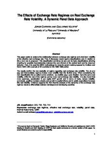
When a country experience a real exchange rate appreciation, goods become more expensive and thereby their competitiveness will decline. An appreciation will occur when the nominal exchange rate appreciates or/and if, the domestic prices is rising faster than the foreign prices. A depreciation will conversely mean a gain in competitiveness (Baldwin and Wyplosz, 2012). This is where the neutrality principle mentioned above becomes relevant, because it assets that the neutral variables will not affect the real variables in the long run. The real exchange should therefore in the long run be unaffected, despite short-term appreciations and depreciations. Short-term changes in nominal exchange rate and price levels domestically or abroad will not have a long-term effect. The PPP thereby imply that the real exchange rate is a constant (Baldwin and Wyplosz, 2014). To examine this principle in practice, we can look at figure (1), Denmark´s nominal and real effective exchange rates the last 37 years.

3

Nominal exchange rate definition: “foreign price of the domestic currency.” (Baldwin and Wyplosz, 2004) Real exchange rate definition: ”Ratio of domestic to foreign good prices expressed in the same currency: λ=EP/P*.4.”( Baldwin and Wyplosz, 2004). 4

8

Anne Cathrine Toft Jørgensen Bachelor thesis

Department of economics 04.05.2015

Nomimal effective vs. real effective krone rate 1977-2014 140 120 100 80 60 40 20

1977 1978 1979 1980 1981 1982 1983 1984 1985 1986 1987 1988 1989 1990 1991 1992 1993 1994 1995 1996 1997 1998 1999 2000 2001 2002 2003 2004 2005 2006 2007 2008 2009 2010 2011 2012 2013 2014

0

Real effective kroner rate

Nominal effective krone rate

Figure (1): Nominal vs. real effective krone rate comparison 1977-2014, calculated in annual averages. Source: (Nationalbanken.statbank.dk, A, 2015), (Nationalbanken.statbank.dk, B, 2015)

The figure shows a seemingly stable real effective krone rate, not being a constant from year to year, but with fluctuation mirroring the nominal krone rate through the years. In the short-run, the story can be quite different, and exchange rates can fluctuate and affect competitiveness and the trade balance (Baldwin and Wyplosz, 2004). A real exchange rate appreciation will make a country less competitive, and result in an external deficit on the trade balance, but eventually the exchange will need to return to its ´normal´ level. This ´normal´ level is called the equilibrium rate, a state where the trade is balanced. In the case of misalignments of the trade balance, and fluctuations from the equilibrium rate, an over-and under-valuation of the exchange rates can happen, which is why PPP is a long-run concept (Baldwin and Wyplosz, 2014). Because the PPP to a degree is an equilibrium rate, it can help when making investment decisions. In the case of a currency being below its PPP, the exchange rate would be expected to appreciate, because investing in the country would become more attractive and vice versa (Lequiller and Blades, 2006). In the case of Sweden, their exchange have been fluctuating around the PPP. This relationship, between the PPP and exchange rate of Sweden is visual graphically in figure [3] in the appendix. This close relationship indicate support to the PPP principle. It is though necessary to consider that fluctuations in the exchange rates can be affected by many other factors, and a simplistic interpretation only on the basis on PPP is not valuable (Lequiller and Blades, 2006). Imbalances can occur all the time, and the correction and return to equilibrium may take a long time. The PPP is not a precise measure, and does not hold in every situation, but it is a good starting point when considering exchange rate behavior over a longer period (Baldwin and Wyplosz, 2014). When having international volume comparisons PPP can also be a valuable tool, because it is statistical constructed whereas exchange rates are a precise measure (Lequiller and Blades, 2006).

9

Anne Cathrine Toft Jørgensen Bachelor thesis

Department of economics 04.05.2015

5.1.2 Short-term affects 5.1.2.1 Interest rates Above it´s established, that money do not have a real long-term effect, but short-term increased money supply can have an influence. An increased money supply will cause interest rates to decline, investing will become more attractive, and stock prices will usually rise. This will result in higher aggregate spending, GDP growth and a decline in unemployment. Investing abroad will become more desirable, which in the case of flexible exchange rate regime will result in a depreciation of the nominal exchange rate. This will affect the real depreciation, export will increase and the country will gain competitiveness (Baldwin and Wyplosz, 2004) Considering a scenario with a fixed exchange rate regime the situation changes. In a situation with continuously rising cost and prices, the real exchange will appreciate, causing loss in competitiveness and the development of a trade deficit. The need for lower interest rates will occur, but because of the country’s commitment to their fixed exchange rate policy, the central bank will need to intervene with other measures (Baldwin and Wyplosz, 2004). They will try to moderate the exchange rate appreciation by selling foreign exchange reserves and buying back their own currency, thereby decreasing the money supply. In the contrary case of a central bank trying to increase its money supply, the defense of their fixed exchange rate will counteract. Thus, a central bank cannot control both the money stock and the exchange rate. In practice, will a country with a fixed exchange rate regime; though be allowed a small room for independent monetary policy (Baldwin and Wyplosz, 2004).

The long-term neutrality of money of was determined above, but in the short-term the conditions of the principle changes. This short-term neutrality of money is called the IS-LM model, and a graphically depiction of the model can be found in figure [4] in the appendix. It depicts the relationship between the interest rate (r) and the real output (Y), with the IS curve (investment savings) and LM curve (liquidity preference-money supply) (Baldwin and Wyplosz, 2004). The IS downward slope represent that a decline in the interest rate will result in an increased demand and output, and it describes the equilibrium condition of the good market. The LM schedule on the other hand is the equilibrium condition of the real money supply on the money market (Baldwin and Wyplosz, 2004). Baldwin and Wyplosz (2004) explains on page 299: “An increase in output generates more demand for money and for credit to which banks respond by raising interest rates, hence the upward slope of the schedule. An increase in the money supply is captures by a rightward shift of the LM schedule.”

10

Anne Cathrine Toft Jørgensen Bachelor thesis

Department of economics 04.05.2015

5.2 Fiscal policy and exchange rates Fiscal policy is another macroeconomic tool governments can use to affect the economy. Here the IS-LM model is relevant again. It explains how fiscal stimuli operates in a small economy (Baldwin and Wyplosz, 2004). A government trying to increase demand in the economy can use fiscal stimuli, done by either changing public spending or the taxation level. This is shown by a rightward shift of the IS curve, shown in figure [4] in the appendix. With the assumption that there is no change in monetary policy, the LM curve will stays the same and the reaction will be an output expansion. This will cause the interest rate to rise, and thereby the budget deficit to increase. This increased government borrowing will then cause upward pressure on the interest rate; though within small economies the interest rated need not the deviate greatly from the worldwide rate. The following development after depend on the countries chosen exchange rate regime (Baldwin and Wyplosz, 2004). Under a flexible exchange rate, an increase in government spending will lead to an increase in the interest rate, and continuously lead to an appreciation of the domestic currency. This appreciation of the domestic currency thereby moderate the immediate effects the fiscal expenditure should have caused on expenditure (Karras, 2011). Under a fixed exchange rate regime, expansionary fiscal policy cannot stand-alone; there will also be a need for expansionary monetary policy. The expansionary monetary policy will be necessary to prevent a domestic currency appreciation. This need for additional expansionary monetary policy is why there from a theoretical perspective should be larger effect from fiscal stimuli under a fixed than under flexible exchange rate (Karras, 2011). Previous theory in this area seem to disagree greatly on the effect of fiscal policy. The Mundell- Fleming theoretical IS-LM model mentioned above makes the prediction, that fiscal stimuli will have an effect on both fixed and flexible exchange rate regime, though a fixed regime will experience greater effects (Karras, 2011). Whereas research by Ilzetki, Mendoza and Vegh (2011) agrees with Mundell-flemming on fiscal expansions effect in a fixed exchange rate regime, they disagree with the effect in a floating exchange rate regime, and finds it completely ineffective (Karras, 2011). Research question 4 explore how Denmark and Sweden used fiscal stimuli to recover from the GFC, and considers if their choice of exchange rate was an influencing factor.

5.3 Choice of exchange rate This paper examines two types of exchange rate regimes, fixed and flexible. In the real world, though exchange rate regime is more diverse, with many hybrids and few extreme cases. All regimes, with the exception of the free-floating exchange rate, will choose a foreign currency to become their anchor. Historically these anchors have typically been the Deutschemark, now replaced by the euro, and the US dollar.

11

Anne Cathrine Toft Jørgensen Bachelor thesis

Department of economics 04.05.2015

5.3.1 Fixed vs. flexible exchange rate 5.3.1.1 .Interest parity The interest parity condition is the property of international financial markets. It occurs when the international financial markets are in equilibrium, and the traders become indifferent between investing domestically and abroad. Capital flows become unnecessary, because the return on domestic and foreign assets is equalized (Baldwin and Wyplosz, 2012). Stated by Baldwin and Wyplosz (2012) page 352 as:

This equation states that if an exchange rate depreciates, foreign assets will thereby become more valuable when measured in the domestic currency, and have the opposite effect if an exchange rate appreciation occurs (Baldwin and Wyplosz, 2012). When considering this in a fixed exchange rate regime as in the case of Denmark, the exchange rate will not have the opportunity to change and thereby the interest rates will fully capture the difference between investing domestically and abroad. If there is a market expectation of a foreign currency to appreciate, the foreign investment will become attractive. The expectation of getting more of their domestic currency when selling the foreign currency will make the country attractive for investors (Baldwin and Wyplosz, 2012). If the opposite is the case, and the foreign capital depreciate over the year, there will be a loss in domestic currency. The loss might be higher than what was gained investing abroad initially at a possible higher foreign interest rate. When considering where to invest it is therefore important, to not only compare the domestic and foreign interest rates. The expected exchange rate develop should be taken into account (Baldwin and Wyplosz, 2012). Applying the interest rate parity to the Euro area, and other countries where the financial market are deeply integrated, a small deviation from the interest parity condition can trigger huge capital flows. It instantly affects the current and expected domestic and foreign interest and exchange rates, and the interest rate parity is re-established. These type of deviations are short-lived, and traders try hard to spot them for a quick return on investment (Baldwin and Wyplosz, 2012). The parity conditions problem is that the expected exchange rate is unknown, and is the expectations of thousands of traders around the world. Therefore, what the condition reveals is the average of trader’s expectations; formulated by Baldwin and Wyplosz (2012) on page 253 as:

12

Anne Cathrine Toft Jørgensen Bachelor thesis

Department of economics 04.05.2015

5.3.1.2 The impossible trinity principle The impossible trinity principle is a contribution to the IS-LM model mentioned above, and helps understand the choice countries face when deciding on an exchange rate regime. It states that only two of the following three features are compatible, they must choose between full capital mobility, fixed exchange rates and autonomous monetary policy (Baldwin and Wyplosz, 2012). Aizenman, Chinn and Ito, (2013) state as follows: “A key message of the trilemma is that the policy makers face tradeoff; increasing one trilemma variable would induce a drop in the weighted average of the other two. A country opting for greater financial openness, for example, must choose whether to forgo exchange rate stability or monetary independence depending on its policy preference.” Relating this principle to Sweden´s and Denmark´s choice of exchange rate regime will shed some light on the trade of they have faced, and their monetary priorities. Sweden´s flexible exchange rate gives them full capital mobility and autonomous monetary policy. They share this approach with the Eurozone, USA, Japan, the UK and Switzerland. This approach is though not within risk. While it gives them full monetary autonomy, any change in their exchange rate can affect their competitiveness (Baldwin and Wyplosz, 2014). When considering Denmark´s “trilemma” choice, they have with their fixed exchange rate policy given up on monetary policy autonomy and only have capital mobility measures (Baldwin and Wyplosz, 2014).

6. Country background 6.1 Denmark´s monetary regime Denmark practices a monetary policy, which aims to ensure price stability through a fixed exchange rate policy. The fixed exchange rate regime was introduced in 1982. Denmark stopped devaluating the krone, and the currency was “locked” to the D-mark (Abildgren, Andersen and Thomsen, 2010). This continued until the introduction of the euro and Exchange rate mechanism (ERM II) in 1999 (Spange and Wagner Toftdal, 2015). Within the euro area, the currency is euro but there is EU countries including Denmark and Sweden who has their own currency. ERM is the heart of the European Monetary System (EMS), an organization all member states joined in 1979. The ERM II helps ensure that there is not excessive exchange rate fluctuations and help create economic stability between the EU currencies. It also ensures smooth operations of the single market, and is an agreement between the ministers and central bank governors of the non-euro area, euro-area member states and the European central bank (ECB) (Ec.europa.eu, 2015). To participate in the agreement there is a number of conditions the countries have to uphold. They have agreed upon a central exchange rate between the countries domestic currency and the euro, where the currency can fluctuate with up to 15 percent above or under the central rate (Spange and Wagner Toftdal, 2015.

13

Anne Cathrine Toft Jørgensen Bachelor thesis

Department of economics 04.05.2015

However, Denmark’s agreement to keep the krone stable against the euro has a much narrower band, with possible fluctuation of 2.25 percent to the central rate of 7.46038. In reality, the band is even tighter, which reduces the risk Danish households and firms incur when dealing with the euro as currency (Spange and Wagner Toftdal, 2015). Figure (2) below shows the exchange rate of the krone against the euro from 19902014, since the 1990 the krone have stabilized on the strong side of its central rate.

Figure (2): Exchange rate of the krone against the euro. Source: (Spange and Wagner Toftdal, 2015, page 52) When the foreign exchange markets are calm, the exchange rate depends mainly on the longer-term interest rates between Denmark and the Euro area. Figure (3) below shows the interest of the Danish national bank and the ECB main refinancing rate. Since 1999 when the euro was introduced, the interest rate between the euro area and Denmark have correlated closely (Spange and Wagner Toftdal, 2015).

14

Anne Cathrine Toft Jørgensen Bachelor thesis

Department of economics 04.05.2015

Figure (3) Monetary policy interest rates in Denmark and he Euro area. Source: (Spange and Wagner Toftdal, 2015, page 51) Despite this close correlation between the monetary interest rates, the Danish national bank regularly asses if there is need for a unilateral response on the rate between the krone and euro. In the case the krone is weakening, the Danish national bank will try to counter act by purchasing kroner against foreign exchange. If this measurement does not have efficient effect on the stabilization of the krone, the national bank have another tool to use, they can unilaterally adjust Denmark’s monetary policy interest rates. An increase in the money market interest rates compared to the euro area e.g., will make it more attractive for investors, boost demand for the kroner and thereby strengthening the currency (Spange and Wagner Toftdal, 2015). The long-term stable Danish krone with narrow fluctuation, have earned the Danish currency high credibility on the market, as well as confidence in the Danish national banks ability to handle monetary policy and foreign exchange rate changes. The participants in the financial market confidence in the krone have reduced the need for interventions by the Danish national bank, the transactions between market participants are typically sufficient. Even in a weak krone scenario, will the market most likely automatically stabilize, because participant will find it more likely for the krone to bounce back than weaken further (Spange and Wagner Toftdal, 2015). Denmark’s fixed exchange rate, shift the focus from monetary policy to be used to stabilizing the business cycle, to the importance of fiscal policy’s influence on the business cycle. The fiscal policy should not contribute to intensifying an economic boom, resulting in a subsequent strong downturn. The Danish national bank warned in the mid-2000s, that because of the lack of spare capacity, Denmark’s fiscal policy was to accommodative. To loose fiscal policy fueled the economic downturn and harmed both household and firms. Another implication of improper fiscal policy can be cyclical fluctuations. Political support for the fixed exchange rate can come to question, which if severe enough can lead to downward pressure on the krone and initiate a unilateral Danish interest rate increase (Spange and Wagner Toftdal, 2015).

15

Anne Cathrine Toft Jørgensen Bachelor thesis

Department of economics 04.05.2015

6.1.1 Danish national bank response options under a financial crisis The Danish national bank have as mentioned above the option of intervening in the foreign exchange market. They have foreign exchange rate reserves consisting largely of euros, deposits in foreign banks and foreign securities with the possibility of selling these or use them as collateral (Spange and Wagner Toftdal, 2015). Denmark’s commitment to fixed exchange rate policy means that monetary policy interest rates, sole purpose is to keep the krone close to its central rate. It is only in the case that it is not possible for the national bank to stabilize the exchange rate of the krone with an intervention in the foreign exchange market, which the national bank will opt to adjusting its monetary policy interest rates. This include the lending rate, rate of interest on certificates of deposits, the current account rate and the discount rate (Spange and Wagner Toftdal, 2015). The most recent example of this happening was in January and February 2015. The krone came under pressure, because huge amount of money was coming into the Danish market. The Danish national bank´s first attempt to stabilize the krone was selling enormous amount of kroner on the market, and thereby building up their foreign exchange rate reserves. This attempt turned out not to be sufficient, therefore the national bank lowered the interest rate to a historical low of 0.75 percent (Skovgaard, 2015). Monetary policy interest rates influence on the krone exchange rate happens through the money market interest rates. The net positions of the banks5, affect which of the monetary policy interest rates that regulates the money market interest rates. In the recent years the general case have been a large positive net position, which means that the sector deposits funds in Denmark´s National bank, which will cause the short-term money market interest rates to follow the rate of interest on certificates of deposit. When the opposite is the case and net position is declining, the money market interest rates will move towards Denmark´s national bank’s lending rate. The krone liquidity will be decreasing, causing the price of krone liquidity to rise. The national bank can influence the net position by numerous factors in the balance sheet, but the most effective is payment to and from the central governments account and intervention by Denmark national bank (Spange and Wagner Toftdal, 2015). Spange and Wagner Toftdal (2015), describes an example of this on page 55: “the net position declines when Denmark´s national buys kroner in the market in order to counter the weakening of the krone. This has a tendency to push up money market interest rates, which has a further stabilising effect on the exchange rate of the krone on top of the direct effect of intervention. “ Denmark’s national banks monetary policy instruments is designed with the goal of flexible and robust implementation of the fixed exchange rate policy, therefore they differ from the other central banks tools including those of the ECB (Spange and Wagner Toftdal, 2015).

5

“The net position is calculated as the monetary policy counterparties’ deposits in current accounts and certificates of deposit less their loans from Danmarks Nationalbank.” (Spange and Wagner Toftdal, 2015, page 55)

16

Anne Cathrine Toft Jørgensen Bachelor thesis

Department of economics 04.05.2015

6.1.3 European central Bank The ECB role is important to consider when examining Denmark’s fixed exchange rate policy. When a country enters the EU, their central bank becomes a part of the euro system, which include the other member states central banks and the ECB (Ec.europa.eu, 2015). The countries thereby give up certain monetary policy measurement, such as currency appreciation and depreciation. The opportunity to manage part of their economies and respond to economic shock is now in the hands of the ECB (Ec.europa.eu, 2015). The ECB uses short-term interest rates to affect aggregate demand, and influence the cost of credit. The Euro system focuses their interest rate on the European Over Night Index Average (EONIA)6. They control the interest rate in two ways explained by Baldwin, R. and Wyplosz, C. (2004), page 445 as follows “(1) The Eurosystem creates a ceiling and a floor for EONIA by maintaining open lending and deposit facilities at pre-announced interest rates. The marginal lending facility means that banks can always borrow directly from the ECB at the corresponding rate; they would never pay more on the overnight market, so the marginal lending rate is in effect a ceiling. (2) The Eurosystem conduct, usually weakly, auctions at a rate that it chooses. These auctions called main refinancing operation, are means by which the ECB provides liquidity to the banking system and the chosen interest rate serves as a precise guise for EONIA.” The Eurosystem strategy to achieve its objective relies on three main elements concerning price stability and risk. The first is economic analysis, which consist on a broad range of reviews and prospects of economic conditions, such as growth, employment, prices, exchange rates and foreign conditions. Monetary analysis is the second and third, which focuses on the evolution of monetary aggregates and credit. These two monetary analysis tools moves in proportion to inflation, and is thereby a medium to long-term mechanism in line with the neutrality principle mentioned above. The short-term to mediumterm indictors therefore come from the economic analysis (Baldwin, R. and Wyplosz, C. 2004). Unlike many other central bank, the ECB does not practice an inflation-targeting strategy. The ECB officially target money growth. They do not want to give an impression of mechanically behavior, but the strategy is similar to inflation targeting with implicit target of 2% definition of price stability (Baldwin, R. and Wyplosz, C. 2004). The Eurosystem takes no responsibility for the exchange rate. The euro is a free-floating currency, with free capital movements, a position that accords well with impossible trinity principle mentioned under the theoretical framework (Baldwin, R. and Wyplosz, C. 2004).

6

”weighted average of overnight lending transactions in the eurozone´s interbank market.” Baldwin, R. and Wyplosz, C. 2004, page 445

17

Anne Cathrine Toft Jørgensen Bachelor thesis

Department of economics 04.05.2015

6.2 Sweden’s monetary regime Sweden became a part of the European Union in 1995, and unlike Denmark and the UK, Sweden did not seek exemption from the EU treaty and was therefore obliged to adopt the euro when it had fulfilled the economic criteria (Fernqvist Svensson, 2006). They participated fully on the two first stages of the EMU, and since 1995 partly in stage three. Despite this Sweden decided, that the decision of adopting the euro would be taken by the Swedish government. In 1997, they decided to postpone the decision of the Euro system and maintain their economic freedom. The Swedish population made the final decision in 2003, they voted no to adapting the euro as currency (Fernqvist Svensson, 2006). In 1992, Sweden was forced to give up their fixed exchange rate regime against the ECU. This action caused turbulence in the foreign exchange market and speculation again the krona. Sweden has since had a floating exchange rate, where the krona is allowed to fluctuate, and will be determined in the foreign exchange market (Riksbank.se, 2011). Sweden monetary policy strategy, have since 1999 been aimed at maintaining price stability, with a specific inflation target. The Swedish Riksbank specified this inflation target to an annual change in consumer price index (CPI) of 2 percent (Monetary Policy in Sweden, 2010). The Riksbank also aims their monetary policy after achieving sustainable growth and high employment, achieved through stabilizing production and employment around long-term sustainable paths. Therefore, the Riksbank practices a flexible inflation targeting, with maintaining inflation stability the main objective of their monetary policy (Monetary Policy in Sweden, 2010). The Swedish Riksdag7, have delegated full responsibility and independence for formulating Sweden’s monetary policy to the independent Riksbank. The aim of the policy is to have a long-term perspective, ensuring credibility and price stability objectives. The Riksbank makes decisions on the repo rate8 in monetary policy meetings, using forecast and scenarios of future economic developments to make their decisions (Monetary Policy in Sweden, 2010). The Riksbank uses an explicit inflation target as their “nominal ancor” to ensure price level stability. By keeping a stable inflation rate, Sweden´s monetary policy aims at contributing to favorable economic development. In a case of high inflation, which often lead to high fluctuations, the effects on the economy can be harmful (Monetary Policy in Sweden, 2010). The Riksbanks mention the following effects “It impairs the economy’s ability to distribute resources efficiently and it becomes more difficult for households and companies to make the right decisions. High and fluctuating inflation also leads to arbitrary and unfair redistribution of income and wealth“. (Monetary Policy in Sweden, 2010, page 9) The Riksbank present regularly goals and their view for a sustainable path for the repo rate. Although this does not mean that, they commit themselves to any specific future monetary policy. They have the ability 7

The Swedish government (Monetary Policy in Sweden, 2010). “The discount rate at which a central bank repurchases government securities from the commercial banks, depending on the level of money supply it decides to maintain in the country's monetary system.” (BusinessDictionary.com, 2015) 8

18

Anne Cathrine Toft Jørgensen Bachelor thesis

Department of economics 04.05.2015

to adjust their monetary policy to changing economic circumstances, so that their forecast for inflation and real economy is well balanced. The forecast of interest rate is not a promise, the future repo rate always have a certain degree of uncertainty (Monetary Policy in Sweden, 2010).

6.3 Sweden and Denmark’s financial situation in recent years. Sweden entered the GFC strong. Their prior banking crisis during the early 1990´s ensured that they were prepared with strong economic institutions. They learned from the previous crisis, and have since introduced far-reaching reforms. They ensured fiscal sustainability reforms and a robust monetary framework, furthermore the country have put a lot of effort in improving labour market and social policies (OECD Economic Surveys: Sweden 2011, 2011). An important variable also to consider when discussion Denmark and Sweden´s financial situation coming into the crisis, is the bursting property bubble Denmark experience in 2007. Denmark had since year 2000 experience an 85 percent increase in housing prices, which lead to an overheated Danish economy (Madsen and I. Pedersen, 2013). The Swedish property prices have increased the same amount between 1990´s and 2007, but have unlike Denmark, not had a decrease. The cause can be Sweden’s lower interest rates and a conversion and reduction the property tax in 2006-2008 (Blomquist, N., Møller Christensen, A. and Haller Pedersen, E. (2010). OECD assess the potential growth of the two countries, to be higher in Sweden. According to the Danish national bank, this is largely due to Sweden history of more disciplined financial politics. Both countries have medium-term plans in their financial politics, but the Swedish government execute its policies more disciplined. Denmark have continuously exceeded the set goal in the public finances, whereas Sweden have been able to stay on target since the end of the 1990´s (Blomquist, N., Møller Christensen, A. and Haller Pedersen, E. (2010). Sweden economy have benefitted by this, and are now on of the few countries in the EU who is not included In the procedure of disproportionate budget deficit. Sweden have also succeed with improving their wage competiveness since mid-1990´s, where the opposite is the case in Denmark. This is mostly due to the difference in the productivity growth in the two countries, which have been 2½ % higher in Sweden. Sweden lower growth in wage is mostly due to them avoiding the same overheating of the economy as Denmark experience in the 2005-2007 (Blomquist, N., Møller Christensen, A. and Haller Pedersen, E. (2010). Consider general wealth of the two countries, Sweden have caught up Denmark in the recent years, and they have now similar gross domestic’s product per citizen when the price difference is considered (Blomquist, N., Møller Christensen, A. and Haller Pedersen, E. (2010).

19

Anne Cathrine Toft Jørgensen Bachelor thesis

Department of economics 04.05.2015

7. The global financial crisis 7.1 Denmark and Sweden’s monetary policy during the financial crisis The recent GFC is different from other prior economic crisis, because the euro have been a stabilizing factor. Prior the euro being introduces, the European countries often competed on devaluating their currencies (Blomquist, N., Møller Christensen, A. and Haller Pedersen, E. (2010).

7.1.1 Denmark As mentioned above, Denmark´s fixed exchange rate regime means that the Danish Nationalbank hand over monetary policy autonomy and monetary measures to the ECB. This is in line with the impossible trinity principle, which states that is not possible to have full capital mobility, fixed exchange rate and monetary policy autonomy. In 2008 during the escalation of the GFC, the ECB started providing liquidity for the euro area banks, causing an increase in the ECB´s interest rate. This caused a negative spread between the Danish Nationalbank lending rate and the ECB´s allotment rate (Monetary review 4th quarter 2009, 2009). The increased spread lead to pressure on the krone, causing a need for the Nationalbank to intervene. To stabilize the kroner they started buying considerable amount of foreign currency in September and October of 2008. The measurement though show insufficient to withstand the pressure on the kroner, forcing the Nationalbank to a unilaterally increase in its monetary policy interest rate, widening the spread to the euro area further (Monetary Policy after the Crisis - Ten Lessons from a Fixed-Exchange-Rate Regime, 2015). The spread between the interest rates became even wider when the ECB on the 8 October 2008, lowered their interest rates by 0.5, with the intensifying GFC as the cause. The Danish Nationalbank continued intervening on the foreign exchange market selling foreign currency for 64 billion kroner in October 2008. They finally managed to stabilize the kroner on 24 October with another increase in the lending rate of 0.5, widening the spread to the ECB rate to 1.75 percent point (Monetary Policy after the Crisis - Ten Lessons from a Fixed-Exchange-Rate Regime, 2015). The kroner slowly strengthened from this point forward, facilitating the Nationalbank to buy back foreign exchange and lower their monetary-policy interest rate (Monetary Policy after the Crisis - Ten Lessons from a Fixed-Exchange-Rate Regime, 2015).

7.1.2 Sweden The GFC reached Sweden in late 2008. Although prior to the crisis eruption, the export in the country had already started to decline, causing their GDP to decline. The consumers became more cautions with consumption, influencing the financial system with rising funding cost and falling financial asset prices (OECD Economic Surveys: Sweden 2011, 2011). During the intensification of the crisis in the second half of 2008, Sweden experienced severe economic downturn. The Swedish economy highly depend on export, and was therefore especially hurt by the fall in international trade. The Riksbank reacted by starting to tighten its policies in September 2008. They aggressively started cutting interest rates from 4.75% to 0.25% by the middle of 2009, them reaching their

20

Anne Cathrine Toft Jørgensen Bachelor thesis

Department of economics 04.05.2015

lowest level since the introduction of the inflation target policy (OECD Economic Surveys: Sweden 2011, 2011). Since July 2010, the Riksbank have been gradually raising their interest rates, but the temporary extraordinary low interest rates was not without risk. The OECD Economic Surveys: Sweden 2011. (2011), page 50 states: “Extraordinary low interest rates, may lead to a distorted allocation of capital and excessive risk-taking (white, 2009). Partly because of the extraordinary nature of these measures it can be difficult to asses when to withdraw them. However, it is advisable to do so slowly and gradually, while carefully monitoring financial developments and having policy options available if there is a deterioration in financing availability.” Sweden abandoned the long-term inflation target of 2% in June 2010, which since the mid-1990 the inflation have been outside the target band about half the time. Although this does not mean Sweden does not have its inflation target under control. They have their long-term inflation expectation anchored and kept it under close control (OECD Economic Surveys: Sweden 2011, 2011).

7.1.3 Exchange and interest rate development The immediate exchange rate reaction to the crisis was different in Sweden and Denmark. Sweden´s kroner depreciated, whereas the Danish kroner appreciated (Blomquist, N., Møller Christensen, A. and Haller Pedersen, E. (2010). Figure (4) below, shows the nominal exchange rate9 prior and during the GFC of the two countries. Though this figure is not representative of the true development in the countries exchange rates, because it is unadjusted and a weighted average value of the price of currency in relation to other currencies (Data.oecd.org, A, 2015). In the figure the two countries exchange rate, seem to have very similar fluctuation. To get a clearer picture of the countries actual development, an examination of the countries PPP and real effective exchange rate are considered.

9

“Nominal effective exchange rate indices are calculated by comparing, for each country, the change in its own exchange rate against the US Dollar to a weighted average of changes in its competitors´ exchange rates, also against the US dollar.” (OECD Economic outlook - Real effective exchange rates, 2014, page 106)

21

Anne Cathrine Toft Jørgensen Bachelor thesis

Department of economics 04.05.2015

Nominal exchange rate 8,000 7,500 7,000 6,500 6,000 5,500 5,000 4,500 4,000 2007

2008

2009

2010 Denmark

2011

2012

2013

2014

Sweden

Figure (4) Nominal exchange rates, total national currency units/US dollar, 2007-2015. Source: Data.oecd.org, A, (2015).

Under long-term effects in the theoretical frame prior in the paper, it is determined that nominal variables do not have an effect on real variables such as growth and unemployment. Therefore, an artificial indicator as the PPP can help reflect the differences in countries price levels that not taken into account by exchange rates (Data.oecd.org, B, 2015). Figure (5) below show the PPP of Sweden and Denmark in the years 20072014.

Figure (5) PPP – Purchasing power parity, total national currency/US dollar, 2007-2014. Source: Data.oecd.org, B, (2015).

22

Anne Cathrine Toft Jørgensen Bachelor thesis

Department of economics 04.05.2015

The left part of the figure include Sweden´s and Denmark´s PPP from 2007-2014, and the percentage decrease or increase from years to year. The Swedish PPP decrease with 1.26% from 2007-2008, but actually increase both from 2008-2009 and 2009-2010 with 1.62% and 0.90%, before again decreasing from 2010-2014. The Danish PPP decreased continuously from 2007-2011 with around 2% and did not start increasing before 2012 with 0,855% and 0,117% in 2013. The right part of the figure show the PPP on a curve. Sweden’s slope increased slightly before finding its constant around 8.8%, almost the same PPP as before the GFC. Whereas Denmark´s slope decrease continuously until 2012, and even with sight increase in 2012 and 2013 is around 0.5-0.6 lower than before the GFC. Another indicator to consider is the real exchange rate. As mentioned above in the theoretical framework, the PPP grounds on the distinction between nominal and real exchange rates. The real exchange rate is a measure of competitiveness, correlating the nominal exchange rate for differences in inflation rates. The real effective exchange rate consider the inflation rates by the use of the consumer price indices. The rates not only takes the market changes in the exchange rate into account, but also the variations in the relative prices for consumers (OECD Economic outlook - Real effective exchange rates, 2014). The real exchange rate insures high degree of comparability across countries and time, and is a valuable measure of short-term competitiveness of countries. (OECD Economic outlook - Real effective exchange rates, 2014). Both of these advantages make the measure very relevant for this specific paper, because it addresses the short-term effects of choice of exchange rates.

Real effective exchange rates 108 106 104 102 100 98 96 94 92 90 88 2007

2008

2009 Denmark

2010

2011

2012

Sweden

Figure (6) Real effective exchange rate – based on consumer price indices, 2010 = 100. Source: (OECD Economic outlook - Real effective exchange rates, 2014)

Figure (6) depict the real effective exchange rate of Sweden and Denmark in a histogram. In 2007 and 2008, the Swedish real effective exchange rate is higher than the Danish with 6.7 and 2.8.

23

Anne Cathrine Toft Jørgensen Bachelor thesis

Department of economics 04.05.2015

This changed drastically in 2009, where Denmark´s real exchange rate continue appreciating and the Swedish depreciate with 9.9, creating a difference between the countries of 10. The Danish appreciating means that during the first years of the GFC, Danish goods became more expensive in foreign currencies, causing a decline in competitiveness. The appreciation does not only mean a decline in export. It also make foreign goods more attractive for the Danish consumers, often leading to an increase in import. Another variable to consider is the interest rate of the two countries. In the theoretical framework, it was established that an increased money supply can have an influence in the short-term, causing interest rates to decline. Lowering the interest rate can influence the aggregate spending, GDP growth, and cause a decline in unemployment of a country. It is therefore a valuable indictor when considering the cause of Sweden’s stronger growth, and the exchange rate policies Sweden and Denmark´s practiced under the GFC.

Short-term interest rates 7 6 5 4 3 2 1

Denmark

Q3- 2014

Q4 - 2014

Q2 - 2014

Q1 - 2014

Q4 - 2013

Q3 - 2013

Q2 - 2013

Q1 - 2013

Q4 - 2012

Q3 - 2012

Q2 - 2012

Q1 - 2012

Q4 - 2011

Q3 - 2011

Q2 - 2011

Q1 - 2011

Q4 - 2010

Q3 -2010

Q2 - 2010

Q1 - 2010

Q4 - 2009

Q3 - 2009

Q2 - 2009

Q1 - 2009

Q4 - 2008

Q3 - 2008

Q2 - 2008

Q1 - 2008

Q4 - 2007

Q3 - 2007

Q2 - 2007

Q 1 - 2007

0

Sweden

Figure (7) Short-term interest rates, total percentage per annum, Q1 2007 – Q4 2014. Source: (Data.oecd.org, 2015).

With the crisis intensifying in the late 2008, the Swedish Riksbank started taken action. They aggressively started easing monetary policy, showed on the declining slope above in figure (7) above. The Danish national bank was limited through their commitment to the fixed exchange rate policy, whereas the Swedish Riksbank had full monetary policy autonomy. The short-term interest rates in Sweden as seen in figure (7) declined continuously, approaching zero through 2009 and most of 2010. With Sweden´s real short-term interest rate being even lower, falling from 21/4 to - 1½ from 2007 to 2009. These rates was much than Denmark´s, the Euroarea’s and the United States (OECD Economic Surveys: Sweden 2011, 2011). Denmark´s interest rates also started declining from the third quarter of 2009, and have held a steady lower level since, between 1.1% -1.6%.

24

Anne Cathrine Toft Jørgensen Bachelor thesis

Department of economics 04.05.2015

Figure (7) show a clear difference in the interest rates levels the two country had during intensive downturn of the economy in 2009 and 2010. Figure [5] in the appendix show the specific percentages the countries experience from 2009-2010, and can further depict the difference. Sweden´s interest rates was very low at 0.2% during 2009, whereas Denmark’s interest was more than 1% above at 1.9% and 1.6%. Sweden´s low interest did not just have a direct effect on the financial sector, they also helped boost the consumers and businesses confidence in the economy, it also increased competitiveness, improving growth even further (OECD Economic Surveys: Sweden 2011, 2011).

8. Analysis The overall research question examined in this paper is; how did Denmark´s fixed exchange rate affect the recovery from the GFC. This paragraph will address the most relevant explanatory factors, divided into four separate sub research questions. The first research question will deal with how the exchange rate policy during the GFC affected Denmark and Sweden´s GDP development. The second research question will explore how the exchange rate policy affected the employment and unemployment during the GFC. The third will examine how the exchange rate during the GFC affected the inflation levels of the two countries. The fourth and last will consider the countries use of fiscal stimuli under the crisis, and if the exchange rate regime was an influencing factor. These specific four explanatory factors chosen because they are all variables that can be affected in the short-term, by changes in either the exchange rate or interest rate. They are therefore relevant for this research paper.

8.1 Sub research question 1 -

How did the exchange rate policy during the financial crisis affect Denmark´s and Sweden’s GDP development?

8.1.1 Data analysis This research question will examine the effect Denmark and Sweden exchange rate regime had on their growth recovery. The analyses will include the real GDP forecast, output gap and potential GDP growth. Both Denmark and Sweden entered the GFC with a large drop in their GDP. The GDP per capita dropped with 2.9821% in Denmark, and 5.2577% in Sweden from 2008-2009. The GDP development following this drop, and during the recovery from the GFC though differed (Andersen, Malchow-MMller and Nordvig, n.d. 2014). According to Andersen, Malchow-MMller and Nordvig, n.d. (2014), Sweden returned to pre-crisis GDP level already in 2010, whereas Denmark in 2014 still had not managed to reach pre-crisis levels. They also argue that monetary regime hold a significant explanatory factor, when considering the recovery of the OECD countries growth following the GFC.

25

Anne Cathrine Toft Jørgensen Bachelor thesis

Department of economics 04.05.2015

They argue: “average annual growth in the 18 countries that did not pursue inflation targeting was -0.48%. For the group of inflation-targeting countries average growth was 1.42%.” (Andersen, Malchow-MMller and Nordvig, n.d. 2014, page 7) “In this paper we have shown that OECD counties with an IT monetary policy framework have systematically outperformed OECD countries with other regimes (predominantly fixed exchange rates) in term of economic growth during the period 2007-12. We have also shown that part of this outperformance can likely be ascribed to the exchange rate flexible of the IT countries and hence to an improved export performance resulting from currency depreciations.” (Andersen, Malchow-MMller and Nordvig, n.d. 2014, page 22)

Real GDP Forecast 8 6 4 2 0 2007

2008

2009

2010

2011

2012

2013

2014

-2 -4 -6 Denmark

Sweden

Figure (8) Real GDP forecast, total annual growth rate in percentage 2007 – 2014. Source: (Data.oecd.org, A, 2015).

Figure (8) show the real GDP forecast of Sweden and Denmark. The real GDP forecast is the growth rate of GDP given in constant prices10. Sweden and Denmark´s growth rate both dropped to -5.1 in 2009, but Sweden returned and exceeded to pre-crisis GDP growth quicker than Denmark. In 2010, Sweden growth rate reached 5.7% against Denmark´s 1.6% and have continuously been higher than Denmark´s since. Denmark on the other hand have fluctuated and have had negative growth rates again in 2012 with -0.8% and in 2013 with -0.1%.

10

“Constant price estimates of GDP are obtained by expressing values of all goods and services produced in a given year, expressed in terms of a base period. Forecast is based on an assessment of the economic climate in individual countries and the world economy, using a combination of model-based analyses and expert judgement. This indicator is measured in growth rates compared to previous year.” Data.oecd.org, F, (2015).

26

Anne Cathrine Toft Jørgensen Bachelor thesis

Department of economics 04.05.2015

Figure (9) OECD Annual Projections: Potential GDP forecast of total economy, and percentage change from previous year of Denmark and Sweden. (Andersen, Malchow-MMller and Nordvig, n.d. 2014) The potential GDP output11 percentage change seen above in figure (9) also depicts the picture of Sweden having stronger growth recovery as above. Denmark´s potential GDP growth rate, have been declining since 2008 and was still in 2014 below pre-crisis levels. Whereas Sweden decreased slightly in 2009 from 2.4214 to 2.0244% before increasing continuously since.

Output gap 2005 - 2014 8 6 4 2 0 2005

2006

2007

2008

2009

2010

2011

2012

2013

2014

-2 -4 -6 Denmark

Sweden

Figure (10) Output gap - deviation of actual GDP from potential GDP as a percentage of potential GDP from 2005 – 2014. Source: (OECD iLibrary, 2015)

11

“Potential gross domestic product (GDP) is defined in the OECD’s Economic Outlook publication as the level of output that an economy can produce at a constant inflation rate. Although an economy can temporarily produce more than its potential level of output, that comes at the cost of rising inflation. Potential output depends on the capital stock, the potential labour force (which depends on demographic factors and on participation rates), the non-accelerating inflation rate of unemployment (NAIRU), and the level of labour efficiency.” (Directorate, 2015)

27

Anne Cathrine Toft Jørgensen Bachelor thesis

Department of economics 04.05.2015

The output gaps are constructed using estimates of potential output12 and can give an indication of the efficiency of an economy. A positive output gap indicates an economy unable to keep up with aggregate demand. The economy growing at an unsustainable rate, and increases the chance of “overheating” the economy. In the case of an economy experience “overheating”, the following average growth will most likely be lower, because of the need for a correction (Koske and Pain, 2015). Koske and Pain (2015) page 51 states: “The output gap provides an indication of potential inflationary pressures within the economy, giving it a potentially important role in the conduct of monetary policy” Figure (10) shows that Denmark´s output gap was continuously bigger than Sweden´s coming into the crisis from 2005-2008. Denmark experienced high output gaps of 5.5% in 2006, 5% in 2007 and 3.1% in 2008. The Danish economy was “overheating” during that period, and have since the GFC been unable to live up to the potential output of their economy. Sweden´s economy was also experiencing high aggregate demand and inflation pressure prior the GFC, though at a lower level than Denmark with 3.6% in 2006, 4.8% in 2007 and 1.9% in 2008. Sweden´s output gap decreased substantially in 2009 to – 4.8, at the same time at their real exchange rate depreciated, indicating a low inflation rate through 2009. OECD argues: “Output have subsequently recovered strongly, with real GDP growing by 4½ per cent in the year to mid2010, and by 6.8% in the third quarter (year-on-year), a good performance compared to most other OECD economies. Even so by fall 2010, GDP was 1% below its pre-recession peak. ” (OECD Economic Surveys: Sweden 2011, 2011, page 20) Part of the cause for the difference in Denmark and Sweden´s GDP growth, might be found in country’s export levels. The Swedish export grew considerably faster than the Danish after 2009. Several indictors can have influenced this. Sweden export is more sensitive to cyclical economic changes, it exist almost of 50% capital goods versus Denmark´s 25%. Sweden have therefore benefited from investment eager countries as Germany and China in recent years. The wage competition have also improved in Sweden, and the average productivity growth have been two and a half times stronger in Sweden than in Denmark. As described under short-term effect in the theoretical framework above, an increased money supply can have an effect. When considering the short-term effects on the GDP, the countries immediate reaction the GFC is important. Sweden´s lowered their interest rates drastically in 2009 when the crisis intensified; according to Baldwin and Wyplosz (2004), this would have influenced several things. Investments would become more attractive, leading to higher aggregate spending and GDP growth. This would also make investing abroad more attractive, causing a real exchange rate depreciation. Sweden would thereby gain competitiveness and their export would increase.

12

“Potential output is derived using a production function method and the NAIRU is obtained from a multivariate model of price inflation” (Koske and Pain, 2015)

28

Anne Cathrine Toft Jørgensen Bachelor thesis

Department of economics 04.05.2015

The interest parity conditions determined that when the real exchange depreciates, it would be more attractive for foreigners to invest in the country. Therefore, Sweden´s real exchange rate depreciation through 2009 would have led to increased exports. Whereas Denmark’s real exchange rate appreciated though 2009, would have caused the country to lose competitiveness and decreased exports (Baldwin and Wyplosz, 2004).

8.1.2 Results Sweden´s real GDP growth rate forecast, returned and exceeded pre-crisis levels quicker than Denmark´s, and have continuously been higher since, reaching 5.7% already in 2010, against Denmark´s lower 1.6%. Sweden´s potential GDP percentage also depicts a picture Sweden´s having a stronger recovery, with only a slight decrease in 2009 from 2.4314 to 2.0244%, before continuously increasing since. The last GDP indicator output gap, shows Sweden´s actual GDP deviated more from the potential GDP than Denmark´s in 2009, before again exceeding Denmark in 2010 an since having a smaller output gap than Denmark.

8.1.3 Sub conclusion The growth indicators analyzes above all indicate Sweden´s economy experienced a faster and stronger recovering in the years after the GFC than Denmark. These finding correspond with the Malchow-MMller and Nordvig, n.d. (2014) research paper, and could indicate that Sweden´s flexible exchange rate regime with inflation targeting, played a role in their strong recovery. Sweden´s higher exports following the GDP growth could also indicate that the chosen exchange rate regime had an influence on the country´s GDP development. Their low interest rate caused in real exchange rate depreciation, making the country attractive for investors, and increased their competitiveness. Denmark´s have struggled with reaching pre-crisis GDP levels. Their potential GDP forecast percentage are still below 2008 levels, and their real GDP growth have continuously been below Sweden´s. Their fixed exchange rate regime limited their reaction options when the crisis intensified, and they had considerable higher interest rates than Sweden. Denmark´s also experienced a real exchange rate appreciation, which would have decreased their competitiveness and exports. Denmark´s slow GDP recovery could indicate that their fixed exchange rate might have been an influential factor, which is in line with previous research in the area.

29

Anne Cathrine Toft Jørgensen Bachelor thesis

Department of economics 04.05.2015

8.2 Research question 2 o

How did the exchange rate policy during the financial crisis affect Denmark and Sweden´s employment and unemployment rate?

8.2.1 Data analysis Sweden took several measures during the crisis, trying to limit long-term unemployment. They are together with Denmark, one of the OECD countries with the highest expenditure on active labor market policies (OECD, 2013). Introducing reform and measures to limit the fall in employment and exits from the labour market, and decreasing the risk of a permanent increase in unemployment (OECD Economic Surveys: Sweden 2011, 2011). Figure (11) below display the employment rate13 of Sweden and Denmark from Q1 2007 – Q4 2014. The graph shows that the Danish employment rate being about 3% higher than Sweden’ with small fluctuation, until Q4 in 2009 where the difference start to decrease. The decrease continues until Sweden starts exceeding Denmark in Q1 2011 with 0.2%. This trend in the data continues, and reaches its highest point in Q1 2014 with Sweden´s employment rate being 2.58% above Denmark´s.

Employment rate 80 78 76 74 72 70

Q 1 - 2007 Q2 - 2007 Q3 - 2007 Q4 - 2007 Q1 - 2008 Q2 - 2008 Q3 - 2008 Q4 - 2008 Q1 - 2009 Q2 - 2009 Q3 - 2009 Q4 - 2009 Q1 - 2010 Q2 - 2010 Q3 -2010 Q4 - 2010 Q1 - 2011 Q2 - 2011 Q3 - 2011 Q4 - 2011 Q1 - 2012 Q2 - 2012 Q3 - 2012 Q4 - 2012 Q1 - 2013 Q2 - 2013 Q3 - 2013 Q4 - 2013 Q1 - 2014 Q2 - 2014 Q3- 2014 Q4 - 2014

68

Denmark

Sweden

Figure (11) Employment rate – total percentage of working age population Q1 2007 – Q4 2014. Source: (Data.oecd.org, B, 2015).

13

“Employment rates are defined as a measure of the extent to which available labour resources (people available for work) are being used. They are calculated as the ratio of the employed to the working age population.” (Data.oecd.org, 2015)

30

Anne Cathrine Toft Jørgensen Bachelor thesis

Department of economics 04.05.2015

The unemployment rate14 of the two countries show similar trends in the data as the employment rate above, with unemployment percentage in Sweden constantly being a few percentages above Denmark’s (Blomquist, N., Møller Christensen, A. and Haller Pedersen, E. (2010). The unemployment rose markedly in both countries when the economic crisis erupted, depicted in figure (12) below. Denmark have significantly lower unemployment rate from Q1 2007 – Q4 2009, about 2% lower than Sweden´s. From quarter one in 2010 the difference start to diminish until quarter two in 2012 where Sweden unemployment shortly is lower than Denmark’s with 0.06%. Sweden unemployment continuously stay on a level of around 8%, whereas Denmark´s unemployment starts declining again creating a 1-2% difference in the countries unemployment rate.

Unemployment rate 10 9 8 7 6 5 4 3 2 1

Q 1 - 2007 Q2 - 2007 Q3 - 2007 Q4 - 2007 Q1 - 2008 Q2 - 2008 Q3 - 2008 Q4 - 2008 Q1 - 2009 Q2 - 2009 Q3 - 2009 Q4 - 2009 Q1 - 2010 Q2 - 2010 Q3 -2010 Q4 - 2010 Q1 - 2011 Q2 - 2011 Q3 - 2011 Q4 - 2011 Q1 - 2012 Q2 - 2012 Q3 - 2012 Q4 - 2012 Q1 - 2013 Q2 - 2013 Q3 - 2013 Q4 - 2013 Q1 - 2014 Q2 - 2014 Q3- 2014 Q4 - 2014

0

Denmark

Sweden

Figure (12) unemployment rate - total percentage of working age population Q1 2007 – Q4 2014. Source: (Data.oecd.org, H, 2015).

Sweden´s lower employment rate until 2011 and higher constant higher unemployment rate are unexpected when considering Sweden´s stronger GDP recovery determined in research question 1. It is also inconsistent with what Koske and pain (2015) argue: “The different measures of output and unemployment gaps for each economy are strongly positively correlated”

14

“Unemployed people are those who report that they are without work, that they are available for work and that they have taken active steps to find work in the last four weeks.” (Data.oecd.org, 2015)

31

Anne Cathrine Toft Jørgensen Bachelor thesis

Department of economics 04.05.2015

Assuming this positive correlative existing, it would be expected that Sweden´s unemployment to be lower than Denmark´s. When considering this difference in the unemployment of the two countries, it is though important to consider the difference in the youth unemployment15. Sweden youth unemployment is generally double the Danish (Blomquist, N., Møller Christensen, A. and Haller Pedersen, E. (2010), and the difference was already existing before the crisis entered, with a difference of 11,66% in 2007 and 12,13% 2008 before the crisis hit (Data.oecd.org, I, 2015). To see a graphical illustration and table of this look figure [6] and [7] in the appendix, which show the youth unemployment of Denmark and Sweden from 2007-2013. Denmark´s lower youth unemployment, is partly caused by intensive youth initiatives. It is not possible for young Danes to obtain public support unless they are somehow within the education system, whereas in Sweden there is not distinguished between this in their unemployment benefits (Blomquist, N., Møller Christensen, A. and Haller Pedersen, E. (2010). After the crisis intensified both countries experience increase in the youth unemployment. Sweden youth unemployment increased with 4.79% from 2008-2009, against 3.8% in Denmark. After 2008 the picture changes and Sweden´s youth unemployment rate starts declining with 0.18% from 2009-2010, with 2% from 2010-2011 before again rising with 0.89% from 2011-2012. Denmark on the other hand continued increasing with 2.14% from 2009-2010 and 0.27% from 2010-2011, until 2012 where it turned around and decrease in 2012 and 2013 with 0.1% and 1.09%.

8.2.2 Result The high youth unemployment rate in Sweden could indicate a partly misleading employment and unemployment rate between Denmark and Sweden. Even though the direct comparison between the countries might be misleading, the fluctuating in the data can still be relevant for examining the relationship between exchange rate regime, output and unemployment rate. Sweden and Denmark´s unemployment rate was both on their highest level in 2009 after the GFC erupted. This happened at the same time as the output gap of both countries reaching low levels of -2.8% for Denmark and -4.8% for Sweden as mentioned above. Sweden´s unemployment declined starting 2010 and through 2011 where the difference between the countries rate was minor. This happened simultaneously as their negative output gap was diminishing, which could indicate that, a positive correlating between output and unemployment rate exist as Koske and pain (2015) argued.

8.2.3 Sub conclusion Sweden´s employment rate quickly starting increasing after the initial downturn following the eruption of the financial crisis in 2009, and exceeded their pre-crisis levels in the fourth quarter of 2014. Whereas Denmark´s employment rate in the fourth quarter of 2014 still was 6.62 percentage below pre-crisis levels. The unemployment of both countries increased, but with continuously lower levels in Denmark even with larger percentage increase in the country than in Sweden. The youth unemployment could be part of the 15

”The youth unemployment rate is the number of unemployed 15-24 years old expressed as a percentage of the youth labor force.” Data.oecd.org, (2015)

32

Anne Cathrine Toft Jørgensen Bachelor thesis

Department of economics 04.05.2015

reason for these contradictory results, with Sweden´s percentage in this age group much higher than Denmark´s. Therefore even though Sweden´s unemployment and youth unemployment are both at a higher level than Denmark´s, their development during the economic crisis could indicate a quicker turnaround than Denmark´s. Their employment rate improved already in the first quarter of 2011 and their unemployment rate increased less than Denmark´s. The fluctuations in the output gap could also indicate that a positive correlating between output and unemployment rate exist, and that the exchange rate regime thereby had an influence.

8.3 Research question 3 o

How did the exchange rate policy during the financial crisis affect the inflation level of Denmark and Sweden?

8.3.1 Data analysis Denmark´s and Sweden inflation approach is different. Sweden pursue a long-term inflation targeting flexible exchange rate regime. The Swedish Riksbank had a long-term inflation target of 2% with fluctuations of ± 1% prior the economic crisis, and their CPI band have averaged at 11/4 since 1995 (OECD Economic Surveys: Sweden 2011. 2011). Denmark´s situation is different. They have limited monetary policy control, which leaves them deeply dependent on the ECB´s monetary policy. The euro area’s medium-term goal is to keep the inflation just below 2 percent, which also helps keep Denmark´s inflation levels low (Spange, M. and Wagner Toftdal, M. 2015). When the Danish economy first started showing signs of overheating, the country dependence on ECB´s monetary policy provided even further stimulus for the economy (Andersen, Malchow-MMller and Nordvig, n.d. 2014) The AS-AD model of aggregate demand and supply mentioned under the theoretical framework, explains the relationship between rate of inflation and cyclical movement of output measured in GDP gap. There is a positive relationship between inflation and growth, thereby an expectation of increased growth leading to increased inflation. The model also states that in recession times the will market shrink, and companies with attempt to maintain their market share by limiting cost and prices (Baldwin, R. and Wyplosz, C. 2004). Therefore, both Sweden´s and Denmark´s inflation rate most likely decreased during the initial downturn in the economy. Sweden´s initial response to the crisis, with low interest rates and increased competitiveness, would also have decreased their inflation rate. Their inflation most likely dropped more than Denmark´s, keeping prices and wages low in the country. As discussed under research question 1 the Andersen, Malchow-MMller and Nordvig, n.d. (2014) research paper argues that countries with an inflation targeting monetary regime and flexible exchange rates as Sweden, weathered the crisis much better than countries with a fixed exchange rate regime. Their analyses also confirms a positive correlation between inflation targeting and growth from a sample of 100 countries.

33

Anne Cathrine Toft Jørgensen Bachelor thesis

Department of economics 04.05.2015

To further explorer this, this research question will analysis of the inflation levels of Sweden and Denmark during the GFC. There as several price indices to measure inflation level of countries, this analysis will include the following: PPI, CPI and the GDP deflator.

PPI 110 105 100 95 90

Q1 - 2007 Q2 -2007 Q3 - 2007 Q4 - 2007 Q1 - 2008 Q2 -2008 Q3 - 2008 Q4 - 2008 Q1 - 2009 Q2 -2009 Q3 - 2009 Q4 - 2009 Q1 - 2010 Q2 -2010 Q3 - 2010 Q4 - 2010 Q1 - 2011 Q2 -2011 Q3 - 2011 Q4 - 2011 Q1 - 2012 Q2 -2012 Q3 - 2012 Q4 - 2012 Q1 - 2013 Q2 -2013 Q3 - 2013 Q4 - 2013 Q1 - 2014 Q2 -2014 Q3 - 2014 Q4 - 2014

85

Denmark

Sweden

Figure (13) PPI – Producer price indices, total 2010 = 100, Q1 2007 – Q4 2014. Source: (Data.oecd.org, G, 2015).

Figure (13) display the PPI of Sweden and Denmark from Q1 2007 – Q4 2014. The data.oecd.org, I, (2015) defines the PPP as: “Producer price indices measure the rate of change in prices of products sold as they leave the producer. They exclude any taxes, transport and trade margins that the purchaser may have to pay. They are often seen as advanced indicators of price changes throughout the economy, including changes in the prices of consumer goods and services.” The inflation differential states that an appreciation in inflation will occur when the nominal exchange rate appreciates or/and if the domestic prices is rising faster than the foreign prices (Baldwin and Wyplosz, 2012). Sweden´s PPI started actively rising through 2008, around the same time as their nominal exchange rate rose from 6.591 to 7.645. The increase continuous until Q1 2009, where it stabilized at a slight higher level fluctuating around 100 (Data.oecd.org, I, 2015). This is although most likely more an expression of Sweden´s short-term nominal exchange rate appreciation occurring in 2009, than an expression of increased inflation. Denmark´s PPI started decreasing in the fourth quarter of 2008, before continuously increasing until second quarter of 2013, stabilizing on a significantly higher level.

34

Anne Cathrine Toft Jørgensen Bachelor thesis

Department of economics 04.05.2015

The short decrease in PPI happened simultaneously with a depreciation of Denmark´s nominal exchange rate in 2008. Denmark’s PPI could indicate that their inflation was increasing throughout the GFC, stabilizing around 107 in 2013. The CPI index is a measure referred to several times throughout the paper, as a measure of inflation. It differs from the PPI, as it is a measure of average price changes for a fixed basket of goods and services. It´s an indicator of price changes through the economy, and a useful tool to measure to price differences across countries. (Data.oecd.org, H, 2015).

CPI 2008 -2013 5 4 3 2 1 0 -1 -2 -3 Denmark

Sweden

Figure (14) Consumer price index – total annual growth rate in percentage, February 2008 – November 2013. Source: (Data.oecd.org, H, 2015).

The CPI in figure (14) express a slight different inflation development than the PPI above. Sweden experienced a drastic downturn in CPI from august until December 2009. The CPI rate was below zero, and happened just following the GFC eruption and the depreciation of their real exchange rate. Thereafter, the inflation level of the country have been rising simultaneously with their real exchange rate, before again decreasing starting 2012. Denmark´s CPI rate also decreased starting 2009, corresponding to the GFC intensifying. The CPI reaches its lowest point in September 2009 with 0.8, simultaneously with Sweden´s lowest point of -1.9. Thereafter the index stabilized at a level fluctuation around two (Data.oecd.org, H 2015). This would indicate Sweden avoided inflation growth when the GFC intensified in 2009, before again slowly rising correlating nicely with their GDP growth during the same time-period. Whereas Denmark seem to have continuously experienced inflation growth throughout the crisis, with rates round 2 percent. The last measure of inflation chosen for this paper is the GDP deflator. Unlike the CPI, the GDP deflator is not based upon a fixed basket of goods and services (OECD iLibrary, 2015).

35

Anne Cathrine Toft Jørgensen Bachelor thesis

Department of economics 04.05.2015

The GDP deflator is a broader indicator of inflation. The OECD factbook 2009: economic, Environmental and social statistics (2009) defines is as follows: “The GDP deflator is an implicit, not an explicit deflator. It is derived by dividing an index of GDP measured in current prices by a chain volume index of GDP, both, typically derived using the expenditure approach. It is therefore a weighted average of the price indices of: goods and services consumer by households, expenditure by government on good, services and salaries, fixed capital assets, changes in investores, export of goods and services, imports of goods and services (minus)”

Figure (15) GDP deflator, percentage change from previous years. Source: (OECD iLibrary, (2015).

Figure (15) show that both Sweden and Denmark entered the crisis with a high GDP deflator in 2008, indicating high inflation in both countries. Sweden´s GDP fell with one after in 2009, but still residing at a quite high inflation level compared to Denmark´s GDP deflator, which fell to 0.5. The GDP deflator is high when the prices of export rise, and/or if the country experience a fall in the value of its currency. Therefore, the cause of Sweden´s high GDP deflator might be the extensive depreciation of their currency occurring during 2009. Conversely, can Denmark low GDP deflator in 2009, might be explained by the real exchange appreciation occurring in 2009, causing a price increase on imports. In 2010 Denmark have a high GDP deflator of 3.2 % and Sweden fall to 1.1. This could potentially again be caused by the real effective exchange rate change the countries experienced. Sweden currency appreciated throughout 2010, whereas Denmark experienced a depreciation of the kroner. The GDP deflator of the two countries, show a different picture of the inflation level than the CPI above. With Sweden experiencing high inflation in 2009, contradictory the results found above. It results might though be a bit misleading, due to the real exchange rate depreciation and appreciation the countries experienced.

8.3.2 Results The different inflation measures of Denmark and Sweden, does not show a clear trend in the data. The PPI of both countries increased throughout the economic crisis, before both stabilizing at a higher level. Only Denmark experiencing a slight decrease in the fourth quarter of 2008. This though seems more likely to be an expression of nominal exchange rate appreciation of the countries, than increased inflation.

36

Anne Cathrine Toft Jørgensen Bachelor thesis

Department of economics 04.05.2015

The CPI indicates a different inflation development than the PPI. The CPI fall drastically for both countries in 2009, corresponding with the GFC intensifying. Sweden´s experiences below zero rates just after the eruption of the GFC, simultaneously with their low interest rates and the depreciation of their real exchange rate. After the initial drop the countries CPI level have been rising, until they both experiences a downturn again staring 2012. Denmark´s CPI reached its lowest point in September 2009 with 0.8, simultaneously with Sweden´s lowest point of -1.9. This could indicate Sweden´s inflation level to be considerable lower than Denmark’s, which could have been an influencing factor in the growth occurring at the time. The GDP deflator show a different inflation picture in 2009 than the CPI. Sweden´s GDP deflator is higher than Denmark´s with 2.4 percentage against 0.5 percentage. These number though be a bit misleading, due to the real exchange rate depreciation and appreciation the countries experienced. The 2010 deflator show similar result as the CPI, with Denmark´s being higher than Sweden´s with 3.2 against 1.1 percentage. This would indicate Sweden avoided inflation growth when the GFC intensified in 2009, before again slowly rising correlating nicely with their GDP growth during the same time-period. Whereas Denmark seem to have continuously experienced inflation growth throughout the crisis, with rates round 2 percent. It is though important to notice that comparative price level measure such as PPI and CPI are dependent on exchange rates and should be analyzed with caution (Data.oecd.org, H, 2015).

8.3.3 Sub conclusion Sweden´s flexible exchange rate policy allowed them to respond immediately to the GFC with several monetary measures, and as discussion in research question 1 it resulted in a quick GDP growth turnaround. The data above could indicate that they also managed to keep their inflation levels low right after the crisis erupted, but simultaneously with their growth rising their inflation levels seems to have risen as well. The analysis point to Sweden´s inflation level being below Denmark´s throughout the crisis. This could indicate that their immediate monetary response, with low interest rates, also affected their inflation rates development. They managed to lower their inflation level considerable during the worst of the economic downturn, keeping prices and wages in check. This can have given them an advantage and helped them in their economic recovery from the GFC. Whereas the result indicate that Denmark´s inflation rate was continuously higher than Sweden´s. This could possibly be connected with their limited monetary control, and indicate a barrier for the economy to recover.

37

Anne Cathrine Toft Jørgensen Bachelor thesis

Department of economics 04.05.2015

8.4 Research question 4 o

How did Denmark and Sweden use fiscal stimuli to recover from the financial crisis, and was choice of exchange rate an influencing factor?

8.4.1 Data analysis The earlier banking crisis in Sweden during the 1990 caused the country to introduce far-reaching reforms to ensure fiscal stability (OECD Economic Surveys: Sweden 2011, 2011). The Swedish government committed themselves to having a strong fiscal framework. They determined a 1% surplus target of GDP over a business cycle, a ceiling for central government expenditures, and a requirement of balanced budgets for the local governments in the country. Their parliament also decides on overall spending across broad areas, without the option of increasing expenditure without reducing on other parameters in the same area (OECD Economic Surveys: Sweden 2011, 2011). Therefore, Sweden´s fiscal policy is another example of their disciplined financial policy as mention above. Sweden entered the crisis having a sound fiscal position, with their gross domestic debt relative low, and with a surplus on their structural budget. This allowed them to inject fiscal stimulus into their economy on top of their automatic stabilizers16, without major effects on their fiscal policy in the long run. Their longterm GDP budget surplus of 1 % gives them room to for fiscal maneuvers and prepares them for any future negative shocks. Sweden’s fiscal position was strong, in better shape than most other OECD countries. (OECD Economic Surveys: Sweden 2011, 2011). The Swedish government pursued expansionary policy, and provided significant support. They introduced government programs to support lending, capital injection programs, income tax and social security contribution reductions, subsidies for house repairs/rebuilding and strengthening active labour market polices (M. Andersen, 2015). These drastic measures caused the financial balance to fall with around 43/4 percentage points of GDP in the period 2007-2010, whereas the euroarea fell with 53/4 and the US with 73/4. This smaller decline was part due to Sweden’s automatic stabilizers being very effective. A change in Sweden´s GDP of 1% was estimated to leading to a 0.55% change in GDP on the budget balance, higher than the OECD average of 0.44% (OECD Economic Surveys: Sweden 2011, 2011). Denmark fiscal policy before the GFC was pro-cyclical, which is different from what was the case in previous upturns in the economy. The fiscal stimuli added pressure on the general economy and on the labour market, instead of counteracting the pressure. Denmark measures to counteract economic overheating is limited due to their fixed exchange rate, therefore making the pro-cyclical policy a possible problem (The Financial Crisis in Denmark, 2013). Despite this fact has Denmark´s fiscal framework strengthened in recent years. The public finances is in seemingly good shape, with strong automatic stabilizers ready to help buffer adverse shocks. The Danish government adopted in 2010 a fiscal Consolidation Agreement to strengthen general government finances.

16

Automatic fiscal stabilizers “Policies or institutions that automatically tend to dampen economic cycle fluctuations in income, employment, etc, without direct government intervention.” (BusinessDictionary.com, 2015)

38

Anne Cathrine Toft Jørgensen Bachelor thesis

Department of economics 04.05.2015

The agreement adding fiscal stimuli of 1.5% of GDP over 2011-2013 (OECD Economic Outlook, Volume 2010 Issue 2, 2010), and additional fiscal stimuli in 2011 of 0.5% of GDP. To compare Denmark and Sweden´s fiscal stimuli during the GFC, Aizenman, J. and Pasricha, G (2013) is considered. The research paper studied patterns of government expenditure stimuli, and collected data on the OECD countries fiscal expenditure growth during the GFC17. Figure (16) show the OECD countries growth in fiscal expenditure from the fourth quarter of 2007 to first the quarter of 2010. The data was split into intervals between Q4 2007 – Q4 2008 and Q1 2009 – Q1 2010. The fiscal response differed significantly across the OECD countries, ranging from -16% in Greece to 12 Portugal. Denmark and Sweden´s annual growth rate as mentioned under research question 1 was similar in 2008 at -0.7% (Data.oecd.org, D, 2015), and their immediate fiscal response was similar as well. The fiscal expenditure for both countries between Q4 2007 – 2008 Q4 grew. Denmark´s a little higher than Sweden, with 1.48% against 1.23%.

Growth Fiscal expenditure OECD countries 14 9

-1 -6

Greece Iceland Ireland Poland Austria Italy N. Zealand Belgium USA Turkey Czech Rep Sweden France Norway Mnetherland Japan Germany Hungary UK Spain Denmark Finland Canada Chile Korea Mexico Australia Portugal

4

-11 -16 2007Q4 - 2008Q4

2009Q1-2010Q1

Figure (16) Government growth rate of pure fiscal expenditure from Q4 2007 – Q4 2008 and Q1 2009 – Q1 2010. Source: (Aizenman, J. and Pasricha, G. 2013)18.

17

All data are in real terms, seasonally adjusted, and it annual rates. The data was collected from national sources and Thomson Financial Datastream, the International Monetary Fund´s (IMF´s) International financial statistics, OECD stat, EuroStat, and DataInsight." Aizenman, J. and Pasricha, G. (2013), page 400. 18 ”The average growth rate is the average over the period of the quarter-on-quarter growth rate.” (Aizenman, J. and Pasricha, G. 2013, page 400)

39

Anne Cathrine Toft Jørgensen Bachelor thesis

Department of economics 04.05.2015

According to Aizenman, J. and Pasricha, G (2013), page 399 the 2008 number´s may not be representative of the real stimuli, they state: “Because of lags in policy formulation and implementation, fiscal expenditures during the period 2009Q1 – 2010Q1 are more likely to reflect the policy response to the recession.” In 2009 the similar annual growth rate continuous, both countries rate decreased with -5.1% Data.oecd.org, D, (2015), but the countries fiscal expenditure growth rate differed significantly. From Q1 2009 – Q1 2010 Sweden fiscal expenditure growth with 1.58%, whereas Denmark´s was significantly higher at 4.1%. To see only see data from Q1 2009 – Q1 2010 illustrated, look at the appendix figure [8]. The OECD economic outlook report from 2009 look further into the effectiveness and scope of fiscal stimulus. The report focuses on the short-term macroeconomic stabilization objectives, and considers the OECD countries fiscal policy response measures (“The Effectiveness and Scope of Fiscal Stimulus”, in OECD Economic Outlook, Interim Report March 2009, 2009)

Figure (17) The size and Timing of fiscal packages 2008-2010. Source: (“The Effectiveness and Scope of Fiscal Stimulus”, in OECD Economic Outlook, Interim Report March 2009, 2009)19 Both countries used similar amount of discretionary fiscal packages20 in the period 2008-2010 to stimulate the economy at -2.5% and -2.8, but the measures used and timing, differed between Denmark and Sweden.

19

“ 1. Cut-off date for information is 24 March 2009. 2. Includes only discretionary fiscal measures in response to the financial crisis. Estimates provided here do not include the potential impact on fiscal balances of recapitalisation, guarantees or other financial operations. They also exclude the impact of a change in the timing of payment of tax liabilities and/or government procurement. 3. Several countries have changed the timing of payment of government procurement and/or tax liabilities. When applying the accrual principle, such measures should not be reflected in the national account data. Still, they affect fiscal balances measures on a cash basis and may have an impact on the economy. They have not been included in the size of fiscal packages.” (“The Effectiveness and Scope of Fiscal Stimulus”, in OECD Economic Outlook, Interim Report March 2009, 2009) 20

“Non-mandatory changes in taxation, spending, or other fiscal activities by a government in response to economic events or changes in economic conditions. Discretionary fiscal policy implies government actions above and beyond existing fiscal policies” BusinessDictionary.com, (2015).

40

Anne Cathrine Toft Jørgensen Bachelor thesis

Department of economics 04.05.2015

Sweden prioritized tax cut higher than boosting the spending of the country, by decreasing the personal income tax. Denmark on the other hand prioritized boosting the spending the country higher than decreasing taxes. Sweden stimuli was spread almost equally between 2009 and 2010, whereas Denmark used 33% in 2009 and 67% in 2010 (“The Effectiveness and Scope of Fiscal Stimulus”, in OECD Economic Outlook, Interim Report March 2009, 2009).

8.4.2 Results Aizenman, J. and Pasricha, G (2013) report indicated that Denmark and Sweden´s fiscal expenditure growth rate during the GFC was similar in 2008 with an increase of 1.48% and 1.23%. In 2009, Denmark was significantly higher at 4.1% against Sweden´s 1.58%. When analyzing the fiscal expenditure growth rates across countries, it is though important to consider it may not be fully representative. The countries fiscal stimuli growth trend before the GFC should considered. Denmark was already pursuing pro-cyclical fiscal stimuli coming into the crisis; this already high expenditure could distort the result (Aizenman, J. and Pasricha, G. 2013). The OECD economic outlook report from 2009 on the effectiveness and scope of fiscal stimulus shows that both countries used similar amount of discretionary fiscal packages. The countries priories was though different, with Sweden prioritizing tax cuts on the personal income tax, Denmark prioritized boosting the spending.

8.4.3 Sub conclusion Denmark and Sweden both used fiscal stimuli to recover from the GFC. Sweden entered the crisis having a sound fiscal position, which allowed them to inject fiscal stimulus into the economy on top of their strong already existing automatic stabilizers. Denmark fiscal policy before the GFC was pro-cyclical, with an already high expenditure on fiscal stimuli. Sweden´s fiscal stimuli growth in percentage is similar to Denmark´s in 2008. This result could though be misleading because of Denmark´s pro-cyclical prior the crisis hitting. In 2009, Denmark´s fiscal expenditure growth was significantly higher than Sweden´s. The net effect on fiscal balance from OECD in the period 2008-2010 shows a slightly different picture. Denmark and Sweden use similar percentage of GDP to stimulate the economy with Sweden´s expenditure slightly higher with -0.3%. The two countries manner and timing of the stimulating differed, Sweden almost equally stimulating their economy in 2009 and 2010, with Denmark only al 33% in 2009 and 67% in 2010. A part of the explanation of Sweden slightly higher stimulus could possibly be their flexible exchange rate. Under flexible exchange rate, an increase government spending will lead to an appreciation of the currency, and moderate the immediate effects of fiscal expenditure. Therefore, it would expected that Sweden would need to use higher amount of fiscal stimuli to achieve economic results.

41

Anne Cathrine Toft Jørgensen Bachelor thesis

Department of economics 04.05.2015

Sweden´s flexible exchange rate regime gives them monetary policy autonomy. They had several supplementary measures to fiscal policy to counteract the GFC, as lowering their monetary interest rate significantly. This could possible explain Denmark higher fiscal stimulus growth in 2009. Denmark fixed exchange policy gives them limited options to stimulate the economy. The monetary policy interest rate sole purpose is to defend the fixed exchange rate, and Denmark have handed full monetary autonomy to the ECB. Therefore, the exchange was an influencing factor for Denmark, and fiscal stimulus an important tool for the country. Sweden flexible exchange rate gave them several reaction options to the GFC. They aggressively supplemented their monetary policy with fiscal policy. Their timing of implementation arguably also seems better, with Denmark waiting until 2010 with a major part of their fiscal stimuli.

9. Evaluation/discussion The cause and effect method used in this paper, have certain challenges that is important to consider when interpreting the result. An often-occurring problem in casual analysis is that other factors than the once analyzed have an influence. In the case of this particular research paper, there are certainly other background factors, which can have had an influence in the economic recovery. Therefore, the results found in the paper are not definitive, but an indication of that the choice of exchange rate can have had an effect. The direction of causation have also been a potential danger zone, because if the direction of causation actually were the opposite, the result found would be misleading (Linderoth, H. and Bentzen, J. 2015). Growth of countries is difficult to measure; therefore, the data presented might not show the entire picture of the growth development in the countries. The choice of the specific explanatory factors in the paper was on the grounds of them being the most significant, and easy comparable between the countries. There was a good amount of data available on most of the explanatory factors, from credible sources like the OECD and the Danish national bank. A problem of data availability though occurred relating to the fourth research question. Credible data on fiscal stimuli was difficult to find, and the automatic stabilizers of the two countries might affect the result in a misleading direction. The Aizenman, J. and Pasricha, G (2013) research paper provided data on the fiscal expenditure growth rate during the GFC. Their result was presented clearly in a table in the paper, and was collected from sources as the international monetary funds, OECD stat, and International Financial Statistics. The data was used in this paper for analyses and graphical illustrations. Though not having the raw data available increases the possibility of misleading results, and therefore should be consider when evaluating the results. The OECD and the Danish national bank are two other primary statistical data source for the paper, and both provide updated credible raw data material. The data was thereafter tabular analyzed or put in graphically illustrations by the use of excel. Therefore, there should be no misleading, or data validity problems with that data.

42

Anne Cathrine Toft Jørgensen Bachelor thesis

10.

Department of economics 04.05.2015

Conclusion

The analysis of the first research question deal with the GDP development during the GFC. The result showed that Sweden did experience stronger and faster recovery in the years following the crisis, and an indication of their flexible exchange rate being an influencing factor. Their monetary policy autonomy enabled them to decrease their interest rates drastically, causing a real exchange rate depreciation. This measure improved their competitiveness, and made the country attractive for investors, increasing their exports considerable. Denmark´s have struggled to recover from the economic crisis, with GDP forecast level still below pre-crisis levels. Their fixed exchange rate limited their monetary policy reaction options, and bound them to follow the EBC´s decisions. The country experienced an appreciation of their currency after the intensification of the crisis, and struggled to stabilize the currency. These finding correspond with Malchow-MMller and Nordvig, n.d. (2014) research paper, and indicate that exchange rate regimes might be an influencing factor on GDP development during a recession. The second research question examines the employment and unemployment development, and if the exchange rate policies of the counties was an influencing factor. The results showed that Sweden generally experience lower employment and high unemployment than Denmark. Though fluctuating in the data during the crisis still showed a picture of Sweden´s economic turnaround being quicker than Denmark´s. The result also confirms the Koske and pain (2015) argument of a correlation between output and unemployment, which could indicate that the difference in the counties exchange rate policy was an influencing factor on the employment and unemployment development. The third research question deals with the inflation development of the two countries, and found that the inflation level in Denmark was continuously higher than in Sweden during the GFC. The result indicate that Sweden´s immediate monetary response, with low interest rates, also affected their inflation rate development. Denmark´s higher inflation level through the crisis could be connected with their limited and slower monetary reaction, and might have been a barrier for their economic recovery. The last research question examines Denmark and Sweden’s use of fiscal stimuli during the GFC, and if the exchange rate was an influencing factor. Both countries used fiscal policy to stimuli their economic during the GFC, though with Denmark´s fiscal growth percentage significantly higher than Sweden´s in 2009. The countries destination for the stimuli and timing though differed. Denmark priorities boosting the spending, whereas Sweden prioritized tax cuts. Sweden timing of fiscal stimuli seem better than Denmark´s, with almost equally stimulus of their economy in 2009 and 2010, with Denmark only at 33% in 2009 and 67% in 2010. The choice of exchange rate regime will affect the amount of fiscal stimuli because under flexible exchange rate, an increase government spending will lead to an appreciation of the currency, and moderate the immediate effects of fiscal expenditure. Therefore, Sweden would need to use more stimuli to obtain the same effects as Denmark. Sweden flexible exchange rate enabled them to use other supplementary measure to fiscal stimuli to counteract the GFC, whereas Denmark´s fixed exchange rate limited them and made fiscal policy an important tool for the country.

43

Anne Cathrine Toft Jørgensen Bachelor thesis

Department of economics 04.05.2015

The results in this paper could indicate that causality exist between Denmark´s fixed exchange and their recovery from the GFC. The results all show Sweden´s having a strong and fast recovery, and that Denmark´s lack of monetary autonomy was a barrier for the country. One the other hand how significant the influence was is difficult to determine, because there are several other background factors influencing the different explanatory variables.

Perspective This paper urge to further research on the relationship between exchange rate regimes and how best to recover from a GFC. Especially fiscal stimuli effect seem to be a controversial topic, worthy and in need for further exploration. Research within this area could be a valuable tool in preparation for any future economic crisis, and help policy makers understand the implication of their decisions. This paper show that decisions made immediately after a GFC erupts can have long-term effect on the economy’s recovery.

44

Anne Cathrine Toft Jørgensen Bachelor thesis

Department of economics 04.05.2015

References Abildgren, K., Andersen, B. and Thomsen, J. (2010). Monetary history of Denmark, 1990-2005. [Copenhagen]: Danmarks Nationalbank. Aizenman, J. and Pasricha, G. (2013). Net Fiscal Stimulus during the Great Recession. Review of Development Economics, 17(3), pp.397-413. Aizenman, J., Chinn, M. and Ito, H. (2013). The 'Impossible Trinity' Hypothesis in an Era of Global Imbalances: Measurement and Testing. SSRN Journal. Andersen, T., Malchow-MMller, N. and Nordvig, J. (2014). (2014) Inflation Targeting, Flexible Exchange Rates, and Macroeconomic Performance Since the Great Recession. SSRN Journal. Andersen, T. and Malchow-MMller, N. (2014). Denmark's Fixed Exchange Rate Regime and the Delayed Recovery from the Global Financial Crisis: A Comparative Macroeconomic Analysis. SSRN Journal. Baldwin, R. and Wyplosz, C. (2004). The economics of European Integration. New York: Mcgraw-Hill Education. Baldwin, R. and Wyplosz, C. (2012). The Economics of European Integration. 4th ed. Berkshire: McGraw-Hill Education. Blomquist, N., Møller Christensen, A. and Haller Pedersen, E. (2010). Den økonomiske udvikling i Danmark og Sverige i de senere år. København: Danmarks Nationalbank, pp.35-46. BusinessDictionary.com, (2015). What are automatic fiscal stabilizers? definition and meaning. [online] Available at: http://www.businessdictionary.com/definition/automatic-fiscal-stabilizers.html [Accessed 23 Apr. 2015]. Data.oecd.org, A, (2015). Conversion - Exchange rate - OECD Data. [online] Available at: https://data.oecd.org/conversion/exchange-rates.htm [Accessed 18 Mar. 2015]. Data.oecd.org, B, (2015). Conversion – Purchasing power parity - OECD Data. [online] Available at: https://data.oecd.org/conversion/purchasing-power-parities-ppp.htm#indicator-chart [Accessed 18 Mar. 2015]. Data.oecd.org, C, (2015). Domestic product - Real GDP forecast - OECD Data. [online] Available at: http://data.oecd.org/gdp/real-gdp-forecast.htm#indicator-chart [Accessed 18 Mar. 2015]. Data.oecd.org, D, (2015). Employment - Employment rate - OECD Data. [online] Available at: http://data.oecd.org/emp/employment-rate.htm [Accessed 18 Mar. 2015]. Data.oecd.org, E, (2015). General government - General government deficit - OECD Data. [online] Available at: http://data.oecd.org/gga/general-government-deficit.htm [Accessed 18 Mar. 2015]. Data.oecd.org, F, (2015). Gross domestic product – GDP – OECD Data. [online] Available at: https://data.oecd.org/gdp/gross-domestic-product-gdp.htm#indicator-chart [Accessed 18 Mar. 2015]. Data.oecd.org, G, (2015). Interest rates - Short-term interest rates - OECD Data. [online] Available at: http://data.oecd.org/interest/short-term-interest-rates.htm [Accessed 18 Mar. 2015].

45

Anne Cathrine Toft Jørgensen Bachelor thesis

Department of economics 04.05.2015

Data.oecd.org, H (2015). Prices - Inflation (CPI) - OECD Data. [online] Available at: http://data.oecd.org/price/inflation-cpi.htm [Accessed 18 Mar. 2015]. Data.oecd.org, I, (2015). Prices - Producer price indices (PPI) - OECD Data. [online] Available at: https://data.oecd.org/price/producer-price-indices-ppi.htm [Accessed 18 Apr. 2015]. Data.oecd.org, J, (2015). Unemployment - Unemployment rate - OECD Data. [online] Available at: https://data.oecd.org/unemp/unemployment-rate.htm [Accessed 14 Apr. 2015]. Data.oecd.org, K, (2015). Unemployment - Youth unemployment rate - OECD Data. [online] Available at: https://data.oecd.org/unemp/youth-unemployment-rate.htm#indicator-chart [Accessed 14 Apr. 2015]. “Denmark: the crisis and beyond”, in OECD Economic Surveys: Denmark 2009, (2009). [online] OECD Publishing. Available at: http://www.oecdilibrary.org.ez.statsbiblioteket.dk:2048/docserver/download/1009191ec003.pdf?expires=1428999702&id=i d&accname=ocid177114&checksum=103457887E87CFB4303A44B872818ABD [Accessed 14 Apr. 2015]. Directorate, O. (2015). OECD Glossary of Statistical Terms - Potential gross domestic product (GDP) Definition. [online] Stats.oecd.org. Available at: http://stats.oecd.org/glossary/detail.asp?ID=2094 [Accessed 28 Apr. 2015]. Dudovskiy, J. (2015). Mundell-Fleming Model as more relaxed version of ISLM - Research Methodology. [online] Research-methodology.net. Available at: http://research-methodology.net/mundell-flemingmodel-as-more-relaxed-version-of-islm/ [Accessed 14 Apr. 2015]. Ec.europa.eu, (2015). What is ERM ΙΙ? – European Commission. [online] Available at: http://eu.europa/economy_finance/euro/adaption/erm2/index_htm [Accessed 10 Feb. 2015]. Fernqvist Svensson, A. (2006). Sweden: A member of the European Union but without the Euro.Futures, 38(2), pp.212-223. Jovanovic, M. (2013). The Economics of European Integration. Cheltenham: Edward Elgar Publishing. Karras, G. (2011). Exchange-Rate Regimes and the Effectiveness of Fiscal Policy. Journal of Economic Integration, 26(1), pp.29-44. Koske, I. and Pain, N. (2015). The Usefulness of Output Gaps for Policy Analysis, OECD Economics Department Working Papers, No. 621,. [online] OECD Publishing. Available at: http://www.oecdilibrary.org/docserver/download/5kzhmnw4337h.pdf?expires=1430210503&id=id&accname=guest&check sum=6B795FCFBD544AEFA58043BB7FCA5A87 [Accessed 28 Apr. 2015]. Laursen, F. (2013). The EU and the Eurozone crisis. Farnham, Surrey: Ashgate. Lequiller, F. and Blades, D. (2006). Understanding national accounts. Paris: OECD. Linderoth, H. and Bentzen, J. (2015). Guidelines for Writing Papers in Descriptive Economics. Madsen, M. and I. Pedersen, F. (2013). Kan svensk økonomi noget som vi ikke kan i Danmark?. Arbejderbevægelsens Erhvervsråd. M. Andersen, T. (2015). Fiscal policy and the global financial crisis. Aarhus Universitet, School of Economics and Management.

46

Anne Cathrine Toft Jørgensen Bachelor thesis

Department of economics 04.05.2015

Monetary Policy in Sweden. (2010). 1st ed. [ebook] Stockholm: Sweriges Riksbank, Available at: http://www.riksbank.se/Upload/Dokument_riksbank/Kat_publicerat/Rapporter/2010/Monetary_policy_20 10.pdf [Accessed 24 Feb. 2015]. Monetary review 4th quarter 2009. (2009). [online] Danmarks nationalbank. Available at: http://www.nationalbanken.dk/en/publications/Documents/2010/01/mon_4qtr_09_web.pdf [Accessed 22 Apr. 2015]. Nationalbanken.statbank.dk, A, (2015). Nationalbankens Statistikbank. [online] Available at: http://nationalbanken.statbank.dk/nbf/106057 [Accessed 6 Apr. 2015]. Nationalbanken.statbank.dk, B, (2015). Nationalbankens Statistikbank. [online] Available at: http://nationalbanken.statbank.dk/nbf/106100 [Accessed 6 Apr. 2015]. OECD Economic outlook - Real effective exchange rates. (2014). [online] OECD Publishing. Available at: http://www.oecdilibrary.org.ez.statsbiblioteket.dk:2048/docserver/download/3013081ec041.pdf?expires=1428079396&id=i d&accname=guest&checksum=1F3341A0B5642F71CB9E3DC0E66E0A8 OECD Economic Outlook, Volume 2010 Issue 2. (2010). [online] OECD Publishing. Available at: http://www.oecdilibrary.org.ez.statsbiblioteket.dk:2048/docserver/download/1210021ec017.pdf?expires=1429697368&id=i d&accname=ocid177114&checksum=774B19868007E27AD44F660A7057BEB5 OECD Economic Surveys Denmark, January 2014. (2014). [online] OECD Publishing. Available at: http://www.oecdilibrary.org.ez.statsbiblioteket.dk:2048/docserver/download/1013211e.pdf?expires=1429695015&id=id&ac cname=ocid177114&checksum=F7DE4A8D18BBD4FC63270EDEFC2B78C5 [Accessed 22 Apr. 2015]. OECD Economic Surveys: Sweden 2011. (2011). [online] OECD Publishing. Available at: http://dx.doi.org/10.1787/eco_surveys-swe-2011-en [Accessed 19 Apr. 2015]. OECD Factbook 2009: Economic, Environmental and Social Statistics. (2009). [online] OECD Publishing. Available at: http://www.oecd-ilibrary.org/economics/oecd-factbook-2009/gdp-deflator_factbook-2009graph26-en [Accessed 23 Apr. 2015]. OECD iLibrary, (2015). GDP deflators | OECD READ edition. [online] Available at: http://www.keepeek.com/Digital-Asset-Management/oecd/economics/oecd-economic-outlook-volume2014-issue-2/gdp-deflators_eco_outlook-v2014-2-table178-en#page1 [Accessed 15 Apr. 2015]. OECD iLibrary, (2015). Output gaps | OECD READ edition. [online] Available at: http://www.keepeek.com/Digital-Asset-Management/oecd/economics/oecd-economic-outlook-volume2014-issue-2/output-gaps_eco_outlook-v2014-2-table172-en#page1 [Accessed 18 Mar. 2015]. OECD (2013) Public expenditure on active labour market policies, Available at:http://www.oecdilibrary.org/employment/public-expenditure-on-active-labour-market-policies_20752342-table9 (Accessed: 21 april 2015) Riksbank.se, (2011). The inflation target | Sveriges Riksbank. [online] Available at: http://www.riksbank.se/en/Monetary-policy/Inflation/Adoption-of-the-inflation-target/ [Accessed 24 Feb. 2015].

47

Anne Cathrine Toft Jørgensen Bachelor thesis

Department of economics 04.05.2015

Skovgaard, L. (2015). Kronen er fortsat under angreb. [online] www.business.dk. Available at: http://www.business.dk/oekonomi/kronen-er-fortsat-under-angreb [Accessed 20 Feb. 2015].

Spange, M. and Wagner Toftdal, M. (2015). FIXED EXCHANGE RATE POLICY IN DENMARK. [online] Nationalbanken. Available at: http://www.nationalbanken.dk/en/publications/Documents/2014/03/Fixed_MON1_2014.pdf [Accessed 10 Feb. 2015]. Straumann, T. (2010). Fixed ideas of money. New York: Cambridge University Press. Tavlas, G., Dellas, H. and Stockman, A. (2008). The classification and performance of alternative exchangerate systems. European Economic Review, 52(6), pp.941-963. “The Effectiveness and Scope of Fiscal Stimulus”, in OECD Economic Outlook, Interim Report March 2009. (2009). [online] OECD Publishing. Available at: http://www.oecdilibrary.org.ez.statsbiblioteket.dk:2048/docserver/download/1208051ec016.pdf?expires=1429792501&id=i d&accname=ocid177114&checksum=426D94A54A204E5C6CA93B141686C721 [Accessed 23 Apr. 2015]. The Financial Crisis in Denmark. (2013). [online] Erhvervs og vækstministeriet. Available at: https://www.evm.dk/english/publications/2013/~/media/oem/pdf/2013/2013-publikationer/18-09-13rapport-fra-udvalget-om-finanskrisens-aarsager/conclusions-and-recommendations-170913.ashx [Accessed 23 Apr. 2015]. Uk.fm.dk, (2015). Danish Monetary and Exchange Rate Policy - Ministry of Finance. [online] Available at: http://uk.fm.dk/portfolio/international-cooperation/eu-economic-and-political-coordination/danishmonetary-and-exchange-rate-policy/ [Accessed 10 Feb. 2015]. Yang, Y. (2015). Chapter 1. [online] Csus.edu. Available at: http://www.csus.edu/indiv/y/yangy/145Ch1.htm [Accessed 3 Apr. 2015].

48