Shruti Gupta Joe Funke Thomas Lipp
Estimating Road Friction for Autonomous Vehicles
INTRODUCTION
12-16-11 CS229 Final Report
system. Data is collected at each time step while the vehicle is operating on a given surface.
Automobiles are connected to the road through the four small areas where tires meet road surface. The friction between these two surfaces defines the limit of the vehicle’s performance, and knowing that friction value allows accurate estimation of the vehicle’s capability. Given a known realtime friction value during operation, existing safety features such as stability control, traction control, and antilock braking systems (ABS) on existing production vehicles could greatly improve [1]. Further, accurate friction estimation is essential for an autonomous vehicle minimizing tracking errors and maintaining stability while operating at the limits of handling.
Further, a maneuver called a ramp steer can be conducted at a given location, the data from which can be post-processed to empirically determine the overall friction of that surface. This was done for five different surfaces covering a range of possible situations, as outlined in Table 1. Note that this approach does not allow us to estimate a continuous friction value, which would be ideal, but categorically selects one of these predetermined values. This is still valuable for identifying changing conditions, such as transitioning from a paved surface to a dirt road, or adapting to worsening road conditions in the face of inclement weather.
Various approaches to friction estimation currently exist, but each has drawbacks making them unattractive to implement. Most approaches require precise vehicle models, in turn requiring a significant time investment determining accurate parameters [2]. Other approaches, such as wheel-slip based friction estimators or lateral dynamics observers, will estimate friction only based on one of longitudinal dynamics (accelerating and braking) or lateral dynamics (turning) [3] [4]. Some approaches, such as those based on steering torque, rely on sensors not always available in production cars [5].
Location Shoreline Lot Bonneville Salt Flats Infineon Raceway Santa Clara Fairground Infineon Raceway Any Location
Road Condition Gravel Salt Wet pavement Dry pavement
Friction Value 0.47 0.68 0.75 0.90
Dry pavement 1.00 Vehicle speeds Unknown near zero Table 1: Friction coefficients for various road conditions
Instead, a machine learning based approach to friction estimation is proposed that can yield a real-time estimate of one of several friction values based on current vehicle longitudinal and lateral dynamics. Such an approach can yield a real-time estimate of friction based only on data available to the vehicle and requires training on existing datasets rather than attempting to build and tune a complete vehicle model.
Supervised learning techniques are implemented with training data constructed from measurement information provided at given time steps labeled with one of the five friction values. A sixth friction category of ‘unknown’ was also added for nearzero vehicle speeds to reduce artifacts (given that there is no way to estimate friction if the vehicle is not moving). FEATURE SETS
SETUP Data was collected on a production Audi TTS fitted with a high precision integrated GPS/INS unit and drive-by-wire capabilities. The vehicle is part of Stanford’s Dynamic Design Lab and is used to research autonomous driving at the limits of handling. Friction estimation is currently not used on the vehicle due to issues previously discussed, but having a realtime estimate of friction could drastically improve the speed and safety of its autonomous driving at the limits of handling.
Initial tests running a soft max algorithm, in which the algorithm was trained on ramp steer data and tested on general non-ramp steer data, resulted in only 11% accuracy. Seeing such high error, the focus was first limited to training and testing only on ramp steer data. This still yielded a training accuracy of only 56%. Such high training error suggests the data may be inseparable with just the basic sensor measurements, motivating the addition of other features relevant to friction estimation.
Available data include measurements from on-board production sensors that yield information such as wheel speeds, steering angle, brake and throttle positions, and engine rpm. These measurements are supplemented by acceleration, velocity, and angular rotation rates provided by the GPS
Estimation methods that determine friction based on lateral dynamics incorporate the tire slip angle , which is the angular difference between the heading of a tire and its velocity [3]. The greater the tire slip angle, the greater the lateral force the tire produces, at least up until the friction 1
limit. Longitudinal based friction estimation techniques instead rely on the longitudinal slip ratio , which is ratio of the difference between the tire’s angular speed and its absolute velocity [4]. The longitudinal force of a tire is similarly related to the slip ratio. The total slip is the square root of the sum of both slips squared.
was conducted using a forward search algorithm in which the feature with the greatest improved generalization error was added at each iteration. To speed performance of the soft max classifier, feature selection was trained on only a fraction of the data (300 samples) as testing showed including more data did not yield markedly improved results. For the soft max algorithm the minimum error was found at 21 features to be 38.68% as seen in Figure 1a. Although far from ideal, it is a significant improvement over the performance without the augmented features. The six most significant features used from feature set 1 were, in order of importance, gear position, side slip, A2 of the front tire, A3 of the front tire, K3 of the front tire and A2 of the rear tire.
Various equations have been proposed relating these tire slips to forces. A linear relationship between slip and force is often a good approximation at low slip angles, while more complicated models depend on complex functions of slip. The Dugoff and Fiala brush tire models, for example, relate forces not to the slips but to terms of =
1+
, Α=
tan 1+
80
raised to the first, second, and third powers [6]. The ‘Magic’ tire formula, on the other hand, relates the force to the tangent of [6]. These forces are proportional to accelerations, which are in turn proportional to friction. Thus the features , tan ( ) , , , , , , were added, where each term has a lumped value for the two front tires and a lumped value for the two rear tires. All of these parameters can be calculated with the basic sensor measurements.
Feature Set 1 Feature Set 2
Percent Error
70 60 50 40 30 20
0
5
10
15 20 Number of Features
25
30
Figure 1a: Feature selection for the soft max classifier training on feature set 1 and 2
Certain data measurements were also removed. Some features were removed because they were highly correlated, but others, such as engine RPM, were removed because they are clearly unrelated to friction; this will be discussed more in the section on feature selection. The test data used for training was collected with various autonomous driving runs spaced over several years, and so leaving such extraneous measurements may allow the classifier to find unwanted structure between the different datasets based on time differences rather than friction differences. Thus four feature sets are referred to in the remainder of this paper, which are outlined in Table 2. Note that feature set 0 is the poor performing data set mentioned earlier and is not used hereafter.
30 Feature Set 1 Feature Set 2
Percent Error
25 20 15 10 5
0
5
10
15
20 25 30 Number of Features
35
40
45
Figure 1b: Feature selection for the GDA classifier training on feature set 1 and 2
Related Extraneous Slip measurements measurements features Set 0 Set 1 Set 2 Set 3 Table 2: Feature sets used for supervised learning algorithms
When feature selection was performed using GDA on feature set 1 the minimum error was found at 24 features to be 9.45% as seen in Figure 1b. The most significant features for GDA were right rear wheel speed, engine rpm, yaw rate, slip of the front tires, brake pressure, and left rear wheel speed. Tables 3a and 3b show the precision and recall of the two analyses. Friction .47 .68 .75 .9 1 Unknown 84% 73% 62% 66% 36% 73% Precision 66% 95% 45% 56% 36% 84% Recall Table 3a: Precision and recall of soft max on feature set 1 Average Precision: 71% Average Recall: 64%
SOFT MAX and GAUSSIAN DISCRIMINANT ANALYSIS Both the soft max and Gaussian discriminant analysis (GDA) classifier were analyzed on the augmented feature set, set number 1, by performing feature selection. Feature selection 2
SUPPORT VECTOR MACHINE
Friction .47 .68 .75 .9 1 Unknown 98% 99% 69% 88% 78% 88% Precision 85% 95% 82% 90% 68% 99% Recall Table 3b: Precision and recall of GDA on feature set 1 Average Precision: 87% Average Recall: 86%
Hoping for better classification results, a support vector machine (SVM) algorithm was implemented using the CSupport Vector Classifier provided by the libsvm package1, which solves the following optimization problem:
The GDA classifier performs better than the soft max classifier which is to be expected given that even with the nonlinear features added, soft max is still going to be poor at classifying a nonlinear phenomenon. The GDA classifier in comparison is less constrained to a linear model. However, neither classifier performs well enough to be acceptable in actual implementation on a car.
1 min ‖ ‖ + , , 2 . .
()
()
+
≥ 1− ,
≥ 0,
= 1, . . . ,
= 1, . . . ,
SOFT MAX and GDA on FEATURE SET 2
where
Unfortunately, parameters such as gear position, which both algorithms rely upon, are known to have minimal correlation to friction. Therefore, in feature set 2, parameters such as gear position, throttle, and engine rpm, which are more likely to classify driver behavior or an autonomous driving algorithm than friction, were removed. As can be seen in Figures 1a and 1b and Tables 3a, 3b, 4a and 4b, performance degraded but only by about 10%. Although this new feature set performs worse it is more likely to be classifying friction than some other feature in the data sets.
This SVM predicts one of two outcomes, so six classifiers were trained for a given dataset, one for each friction value. Once trained, each classifier predicts the likelihood that a given dataset may be labeled with its friction value, and the highest probability value is assumed. Thus any number of friction values could be used for classification, simply entailing a classifier for each value. The features were normalized to mean zero and standard deviation 1 to improve performance and reduce computation time. Normalization resulted in improvements on the order of 2.8 times the accuracy in 54% of the computation time2.
Friction .47 .68 .75 .9 1 Unknown 66% 71% 40% 48% 100% 99% Precision 79% 71% 22% 54% 1% 99% Recall Table 4a: Precision and recall of soft max on feature set 2 Average Precision: 71% Average Recall: 58%
is the training data and
are the friction values.
Training on increasing fractions of the ramp steer data, from 1/400 to 2/3 of the data, SVM was run with the four provided kernels: linear, polynomial, radial bias, and sigmoid. Figure 2 plots the resulting generalization error using feature set 2 and the default values for each of the kernels. The polynomial kernel produced the lowest error for every training amount, and the performance of the respective kernels against one another remained the same across all three feature sets. Some basic parameters were tweaked between the different kernels, but the polynomial kernel consistently performed best. This is consistent with the knowledge that friction is highly nonlinear in the parameters measured. This ability to handle nonlinear features allows the SVM with polynomial kernel to perform several orders of magnitude better than either soft max or GDA and even the SVM with linear kernel. The irregularities
Friction .47 .68 .75 .9 1 Unknown 98% 93% 47% 60% 71% 87% Precision 83% 94% 58% 66% 43% 98% Recall Table 4b: Precision and recall of GDA on feature set 2 Average Precision: 76% Average Recall: 74% Using feature set 2, the minimum error the soft max algorithm achieved was found at 15 features to be 43.63%. The most significant features for the soft max algorithm were pitch angle, longitudinal velocity, side slip, A3 of the rear tires, K2 of the front tires, and the velocity of the right front wheel. For the GDA algorithm using feature set 2, the minimum error was found at 14 features to be 18.45%. The most significant features for GDA were right rear wheel speed, roll angle, lateral acceleration, A2 of the rear tires, break pressure, and K2 of the rear tires. These features are more likely to be correlated with friction.
1
Available at www.csie.ntu.edu.tw/~cjlin/libsvm/. Training on 2/3 of the ramp steer data with feature set 2 using SVM polynomial kernel, d=3, c=0
2
3
in the trends for each kernel seen in Figure 2 can likely be attributed to the random sampling of data in small sizes.
kernel is able to create features that can approximate or even perform better than the nonlinear features. Reducing the size of the feature set is advantageous when moving the algorithm onto the vehicle for real-time calculation, since feature set 3, with about half the number of features, requires less computation time from the on-board computer.
Test Error of Different SVM Kernals (Feature Set 2) 0.45
-3
0.4
7
Test Error as Polynomial Degree Varies
x 10
Feature Set 1 Feature Set 2 Feature Set 3
0.35 0.3
Linear Kernal Polynomial Kernal Radial Basis Kernal Sigmoid Kernal
0.25
5
Generalization Error
Generalization Error
6
0.2 0.15 0.1
4
3
2 0.05 0
1 1
2
3
4
5 6 Training Data Size
7
8
9
10 0
Figure 2: Testing different SVM kernels
3
4
5
6 7 8 Polynomial Degree
9
10
11
12
Figure 3: Varying polynomial degree
The polynomial kernel is ( , )=
2
1
GENERALIZING THE DRIVING MANEUVER + So far the analysis was restricted to ramp steer data sets because of their ease of data collection and analysis: they can be easily run, and once collected, they represent a variety of vehicle states in a relatively small amount of data. However, generalization of these results to any driving situation, such as driving in an oval, would be ideal. To test if ramp steer data was general enough training data to generalize to any driving maneuver, SVMs with polynomial kernels d=7, c=1 were trained on ramp steers and tested on ovals. The results for feature set 3 are displayed in Table 55. These results indicate that ramp steers are not general enough to use as training data for a classifier to predict friction during any driving maneuver, which would have been ideal; instead, the algorithm must be trained with the maneuvers that the vehicle may experience.
where N is the number of features and c and d are parameters of the kernel. A value for d was found by training and testing on ramp steer data. A non-zero c value was chosen so that polynomial terms of order less than d would also be included in the kernel. Tests showed that as long as c was greater than 1 its value did not have a significant impact on performance. Increasing the degree of the kernel caused results to fluctuate from one training size to the next, likely due to numerical errors building up as small numbers are raised to large powers. This especially became prevalent with d>9. Based on this, the analysis of prospective d values was restricted to values less than or equal to 9. The results from varying degree d while training on 2/3 of the ramp steer data with feature sets 1 through 3 are shown in Figure 3. Given the comparable performance of the polynomial of degree 7 and degree 8, and the degradation of performance with feature set 1 on the polynomial of degree 8, the polynomial of degree 7 was selected. A polynomial kernel of degree 7 should also be less susceptible to numerical errors from raising small numbers to high powers.
Training Testing Error Ramp Steer Ramp Steer data 0.03% Ramp Steer Oval data 20.75% Ramp Steer + Oval Oval data 0.38% Table 5: Training and testing on different maneuvers As long as the algorithm is trained on data from ovals as well as ramp steers, it does a good job of predicting friction during both maneuvers, as shown in Figure 44. This ramp and oval trained algorithm was implemented at the Santa Clara site, where the vehicle ran ovals around the testing site. The resulting friction estimation at each time step is included in
Given the high performance of the SVM the slip values for feature set 3 that were added for feature sets 1 and 2 were removed. The comparable performance even with these features removed suggests that the SVM with the polynomial 4
Figure . Assuming a uniform friction value of 0.9, the algorithm returned a 10.67% error. However, this site has significant gravel patches, pot holes, and broken concrete, so the true friction values for each point in time are unknown but at times certainly could be lower than 0.9, so the true accuracy of the algorithm is likely higher than 10.67%.
If this limitation is met, however, the classifier is capable of predicting friction values in real-time. However, the best algorithm is not always consistent in its prediction results from data set to data set, even if the data are from the same surface, which is likely due to a lack of diversity in training data. Going forward, training the classifier on a more diverse set of data would be ideal, likely starting with ramp steers. Next steps also include exploring other driving maneuvers and seeing how well the algorithm predicts friction for those scenarios.
Ramp and Oval Data (Feature Set 3) 0.2 Ramp Data Only Ramp + Oval Data
0.18 0.16
Generalization Error
0.14
[1] van Zanten, Anton. Evolution of electronic control systems for improving the vehicle dynamic behavior. Proceedings of the International Symposium on Advanced Vehicle Control (AVEC), pp. 7-15, 2002. [2] R. Rajamani, D. Piyabongkarn, J. Lew, K Yi, and G. Phanomchoeng. Tire-road friction-coefficient estimation. IEEE Control Systems Magazine, pp. 54-69, August 2010. [3] J.-O. Hahn, R. Rajamani, and L. Alexander. GPS-based real time identification of tire-road friction coefficient. IEEE Trans. Contr. Syst. Technol., vol. 10, no. 3, pp. 331–343, May 2002. [4] C. Lee, K. Hedrick, and K. Yi. Real-time slip-based estimation of maximum tire-road friction coefficient. IEEE Trans. On Mechatronics, vol. 9, no. 2, pp. 454-458, June 2004. [5] J. Hsu, S. Laws, C. Gadda, and C. Gerdes. A method to estimate the friction coefficient and tire slip angle using steering torque. IMECE, 15402, November 2006. [6] Rajamani, Rajesh. Vehicle dynamics and control. 2nd Edition, SAE International, Warrendale PA, 2006.
0.12 0.1 0.08 0.06 0.04 0.02 0
1
2
3
4
5 6 Training Data Size
7
8
9
10
Figure 4: Prediction accuracy on ramp steer and oval maneuvers 1
Estimated Friction Value
.9 .75 .68
.47
unknown 0
2000
4000
6000 8000 Time Step
10000
12000
Figure 5: Estimated friction values for oval driving at Santa Clara Fairground CONCLUSIONS A way to estimate friction from basic vehicle information available from stock vehicle sensors and an additional GPS system was found. While soft max and GDA classifiers do not perform well, a polynomial kernel SVM produces excellent results. Training and testing on ramp steer maneuvers works well, but training on ramp steers and predicting friction while running other maneuvers, such as ovals, does not work well, indicating that this approach requires training on all possible driving maneuvers that may occur during friction estimation. 5