SERIES ⎜ ARTICLE

Error Correcting Codes 1. How Numbers Protect Themselves Priti Shankar Linear algebraic codes are an elegant illustration of the power of Algebra. We introduce linear codes, and try to explain how the structure present in these codes permits easy implementation of encoding and decoding schemes. Introduction Priti Shankar is with the Department of Computer Science and Automation at the Indian Institute of Science, Bangalore. Her interests are in Theoretical Computer Science.

1

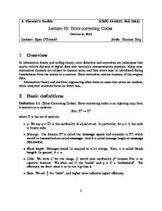
At the time of the writing of this article the Galileo space probe launched in 1989, has sent back stunningly sharp images of Ganymede, Jupiter’s largest moon. The images, which came from Galileo’s flyby of the moon on June 26–27 1996 are reported to be 20 times better than those obtained from the Voyager.

26

Many of us who have seen the pictures sent back by the spacecraft Voyager 2, have been struck by the remarkable clarity of the pictures of the giant gas planets and their moons. When Voyager sent back pictures of Jupiter’s moons and its Great Red Spot in 1979, it was six hundred and forty million kilometres from Earth. A year later, it sent close up shots of Saturn’s rings, clear enough to see the rotating spokes of the B-ring. In 1986 when transmitting near Uranus, Voyager was about 3 billion kilometres away, and in 1989, after being 12 years on the road to the outer reaches of the solar system, and nearly 5 billion kilometres away from Earth, it was able to transmit incredibly detailed, perfectly focused pictures of Triton, Neptune’s largest moon. This great feat was in no small measure due to the fact that the sophisticated communication system on Voyager had an elaborate error correcting scheme built into it. At Jupiter and Saturn, a convolutional code was used to enhance the reliability of transmission, and at Uranus and Neptune, this was augmented by concatenation with a Reed-Solomon code. Each codeword of the Reed-Solomon code contained 223 bytes of data, (a byte consisting of 8 bits) and 32 bytes of redundancy. Without the error correction scheme, Voyager would not have been able to send the volume of data that it did, using a transmitting power of only 20 watts1.

RESONANCE ⎜ October 1996

,, \ SERIES

I ARTICLE

The application of error correcting codes in communication systems for deep space exploration is indeed impressive. However that is only part of the story. Error correcting codes are used extensively in storage systems. If you have a CD player at home, then you have a data storage system with error correction, that uses Reed-Solomon codes. A typical audio CD can hold up to seventy five minutes ofmusic. The music is represented digitally, using zeros and ones. In fact, it takes about one and a half million bits to represent just one second of music. These bits are represented by pits on the mirror-like surface on one side of the disk. T4e pits have an average length of about one micron, and are recorded along a spiral track which is about 0.5 microns wide. Such microscopic features are susceptible to all kinds of errors scratches, dust, fingerprints, and so on. A dust particle on the disk could obliterate hundreds of bits, and without error correction, cause a blast like a thunderclap during playback. However, around two billion bits are added, to protect the six billion or so bits on the disk. As a result, even if there is a 2mm long scratch(which corresponds to an error that spans around 2400 consecutive bits), the quality of music during playback will be as good as the original.

Error correcting codes are used in communication and storage systems.

There is a conceptual kinship between the two examples here. Both involve the handling of data which may be corrupted by noise. There is a sourceof information, an unreliablemedium or channelthrough which the information has to be transmitted, and a receiver.In the spacecraft, the medium is space, and the signals transmitted are subject to atmospheric disturbances, in addition to radiation. In the case of the CD, the communication is in time rather than in space, and the unreliable medium is the recording surface. We owe to the genius of Claude Shannon, one of the finest scientific minds of this century, the remarkable discovery that reliable communication is possible, even over an unreliable medium. In 1948,Shannon, then a young mathematician, showed that arbitrarily reliable communication is possible at any rate

RESONANCEI October 1996

Reed-Solomon

codes

facilitated the transmission of pictures like this one from Voyager 2, a view of Uranus seen from one of its moons, Miranda,_

27

SERIES I ARTICLE

Figure 1 Scheme for communicating reliably over an unreliable channel.

Sender

lllel8age

>I

Encoder

I

cadell'fOrd >1 Channel

I.codeword ) Receiver garbled > IDecoderl estimated meuage

below something called the channelcapacity.Roughly speaking, the channel capacity is its ultimate capability to transmit information, and one can push the channel to this limit and yet correct all the er,rorsit makes using error correction. The illustration in Figure1 shows Shannon's scheme for communicating reliably over an unreliable channel. The message is sent over the channel, but before it is sent it is processed by an encoder.The encoder combines the messagewith some redundancy, in order to create a codeword.This makes it possible to detect or correct errors introduced by the channel. At the receiver's end, the codeword, which may be corrupted by errors is decodedto recover the message.

Let us assume that information is transmitted in terms of binary I digits or bits. Given any sequence of k message bits, the encoder II must have a rule by which it selects the r check bits. This is called the encodingproblem. The k+r bits constitute the codeword, and n

= k +r

is the block length of the codeword.

There are

zn binary sequences of length n, but of these, only Zk are I codewords, as the r check bits are completely defined (using the I encoding function), by the k message bits. The set of Zk I codewords is called the code.When one of these codewords is I transmitted

over the channel, it is possible that anyone of the 2ft

I

binary sequences is received at the other end, if the channel is I daudeShannonshowed

sufficientlynoisy.The decodingproblemisthen to decide which ·

that any communication process can be rendered reliable by adding protectiveredundancy to

one of the Zkpossible codewords was actually sent.

the Information to be transmltled.

Among the simplest examples of binary codes, are the repetition codes.These have k=l, r arbitrary, depending on the degree of

28

Repetition

Codes

RESONANCE I October

1996

SERIES ⎜ ARTICLE

Claude Elwood Shannon was born in Gaylord, Michigan on April 30, 1916. His undergraduate work was in electrical engineering and mathematics at the University of Michigan, and he got his PhD in 1940 at the Massachusetts Institute of Technology. A year later he joined the Bell Telephone Laboratories in Princeton, New Jersey. Shannon’s landmark paper ‘A mathematical theory of communication’ appeared in 1948. Essentially it said that it was possible to communicate perfectly reliably over any channel however noisy it may be. The result was breathtakingly original. Gradually, mathematicians and engineers began to realize that the problems of encoding, transmission, and decoding of information, could be approached in a systematic way. Thus was born a brand new field,which has since been greatly enriched by contributions from others.

error protection required, and n = r+1. For example, if r = 4, we have a repetition code in which the symbol to be transmitted is repeated five times. There are two codewords, the all-zero codeword and the all-one codeword. At the receiving end, the decoder might use a majority vote of the bits to decide which codeword was actually transmitted. If there are more zeros than ones, then it decides that the all-zero codeword was sent, otherwise it decides that the all-one codeword was sent. If the channel noise flips more than half the bits in a codeword, then the decoder will commit a decoding error, that is, it will decode the received sequence into the wrong codeword. However, if less than half the bits are garbled during transmission, then the decoding is always correct. Thus, if n = 5, then two or fewer errors will always be corrected and the code is said to be double error correcting. It is easy to see that for arbitrary odd n, any combination of (n-1)/2 or fewer errors will be corrected. If the code has a long block length, and if channel errors occur infrequently, then the probability of a decoding error is very small. Let us compute the probability that a bit is decoded wrongly using a scheme where each bit is repeated five times. Suppose we assume that the probability of a one being received as a zero or a zero being received as a one is p. This is sometimes called the raw bit error probability. We can compute the probability that a bit is decoded wrongly, using the decoding scheme where

RESONANCE ⎜ October 1996

29

SERIES ⎜ ARTICLE

the majority vote is taken. This is the probability that either three, four, or five bits are flipped by the channel. If we call this probability Pe , then this is given by Pe = probability(3 errors)+ probability(4 errors)+ probability (5 errors) Let Ni be the number of ways in which i bits can be chosen out of 5 bits. Pe = N3 p3 (1-p)2 + N4 p4 (1-p) + N5 p5 =10p3 (1-p)2+ 5p4 (1-p)+ p5. If p is 0.1 we see that Pe is about 0.0086, giving a significant improvement. Smaller values for Pe can be obtained by increasing the number of repetitions. Thus we can make Pe as small as desired by increasing the length of the code. This is not particularly surprising, as all but one bit of each codeword are check bits. (Shannon’s result promises much better). The information rate R of a code is the ratio k/n and is a measure of the efficiency of the code in transmitting information. The repetition codes of block length n have rate 1/n, and are the simplest examples of linear algebraic codes.

The Parity Check Matrix Though the repetition codes have trivial encoding and decoding algorithms,they are not totally uninteresting. In fact, since they are so simple, they provide an easy illustration of a key concept in linear codes - the parity check matrix and the role that it plays in the decoding process. We can consider each codeword to be a vector with n components in the field with the two elements 0 and 1 (We will refer to this field as F2 ). The set of all vectors of length n over F2 is a vector space with 2n vectors. The code is a subspace with 2k vectors. In the case of the repetition code of length five described

30

RESONANCE ⎜ October 1996

SERIES ⎜ ARTICLE

above, the vector space has thirty two vectors, that is, all combinations of five bits, and the code has two vectors. In a linear algebraic binary code, the sum of two codewords is also a codeword. Addition of vectors is defined as componentwise modulo 2 addition. In modulo 2 addition, 1+1=0 and 0+1=1+0=1. Thus the sum of vectors 10101 and 11001 is 01100. With modulo 2 addition, the sum and difference of two vectors is the same, as +1 is the same as –1 modulo 2. We write this as 1 ≡ –1 (mod 2). The symbol ≡ is read as is congruent to. If two bits are the same then their sum is congruent to 0 modulo 2. We follow a convention where the bits are indexed consecutively from left to right beginning with 0. Let c = (c0 , c1 , ... c4 ) be a codeword for the length 5 repetition code. The following four rules for a codeword completely specify the code. 1. The zeroth and first bits are the same. 2. The zeroth and second bits are the same. 3. The zeroth and third bits are the same. 4. The zeroth and fourth bits are the same. The above rules are equivalent to the following four equations c0 + c1 c0 + c2 c0 + c3 c0 + c4

≡ 0 (mod 2) ≡ 0 (mod 2) ≡ 0 (mod 2) ≡ 0 (mod 2)

The equations above can be expressed in matrix form as

⎡1 ⎢1 ⎢ ⎢1 ⎢ ⎣1

1 0 0 0⎤ 0 1 0 0⎥⎥ 0 0 1 0⎥ ⎥ 0 0 0 1⎦

⎡ c0 ⎤ ⎢c ⎥ ⎢ 1⎥ ⎢c2 ⎥ ⎢ ⎥ ⎢c3 ⎥ ⎢⎣c4 ⎥⎦

RESONANCE ⎜ October 1996

⎡0 ⎤ ⎢0 ⎥ = ⎢ ⎥ ⎢0 ⎥ ⎢ ⎥ ⎣0 ⎦

31

SERIES ⎜ ARTICLE

In medical parlance, a syndrome is an indicator of underlying disease. Here too, a non zero syndrome is an indication that something has gone wrong during transmission.

The first matrix on the left hand side is called the parity check matrix H. Thus every codeword c satisfies the equation

⎡0 ⎤ ⎢0 ⎥ H cT = ⎢ ⎥ ⎢0 ⎥ ⎢ ⎥ ⎣0 ⎦ Therefore the code can be described completely by specifying its parity check matrix H. Problem What is the parity check matrix for a binary repetition code with two message bits, each of which is repeated three times?

Decoding The decoder has to eventually answer the following question: Given the received pattern, what is the most likely transmitted codeword? However, it turns out that it is easier to focus on an intermediate question, namely: What is the estimated error pattern introduced by the noisy channel? For if r is the received pattern, and e is the error pattern, and addition between patterns is defined componentwise modulo 2, then r = c + e, and therefore, c = r+e. (In the binary case, r+e = r – e). If the receiver gets the pattern r and he forms the product H rT, then this is, HrT = HcT + HeT = HeT. In general, this is not the all zero column vector, though of course, if the error pattern corresponds to a codeword, it will be the all zero vector. This product is of key importance in decoding and is called the syndrome. Note that the sydrome bits reveal the pattern of parity check failures on the received codeword. In medical parlance, a syndrome is an indicator of underlying disease. Here too, a non zero syndrome is an indication that something has gone wrong during transmission. We can carry the analogy even further. A syndrome does not point to an

32

RESONANCE ⎜ October 1996

SERIES ⎜ ARTICLE

unique disease. Here, the same syndrome can result from different error patterns. (Try the error patterns 11000 and 00111, for instance). The job of the decoder is to try to deduce from the syndrome which error pattern to report. Suppose a single error has occurred during transmission. Then the error pattern will have a single 1 in the position in which the error has occurred and zeros everywhere else. Thus the product HeT will be the ith column of H if i is the error position. Since the five columns of H are all distinct, each single error will have a distinct syndrome which will uniquely identify it. If the fifth bit is in error, the error pattern is 00001, and the syndrome will be the column of H with entries 0001.

A syndrome does not point to an unique disease. Here, the same syndrome can result from different error patterns.

What happens if there is a double error? Continuing the line of argument above, each of the two 1’s in a double error pattern will identify an unique column of H and therefore the syndrome for a double error pattern, with 1’s in positions say i and j, will just be the mod 2 sum of columns i and j of H. The number of double error patterns here is ten. (This is the number of ways in which 2 bits can be chosen from 5). The list of syndromes for the ten double error patterns is:1110,1101,1011,0111,0011,0101, 1001,0110,1010,1100. That for the five single error patterns is:1111,0001,0010,0100,1000. We can see that every single and double error pattern has a distinct syndrome that uniquely identifies it. The syndromes for the single and double error patterns, together with the all zero syndrome, account for all the sixteen combinations of the four bits of the syndrome. Thus the syndrome for any error pattern with three or more 1’s, will be the same as the syndrome for some error pattern with up to two 1’s. For example, 00111 gives the same syndrome as 11000. How does the decoder decide which error pattern to report? Under the assumption that the raw bit error probability is less than 1/2, and that bit errors occur independently of one another,

RESONANCE ⎜ October 1996

33

SERIES ⎜ ARTICLE

the more probable error pattern is the one with fewer 1’s. Thus the decoder follows what is known as a maximum likelihood strategy and decodes into the codeword that is closer to the received pattern. (In other words, it chooses the error pattern with fewer 1’s). Therefore, if a table is maintained, storing the most likely error pattern for each of the sixteen syndromes, then decoding consists of computing the syndrome, looking up the table to find the estimated error pattern, and adding this to the received message to obtain the estimated codeword. For most practical codes, storing such a table is infeasible, as it is generally too large. Therefore estimating the most likely error pattern from the syndrome is a central problem in decoding. Problem How does syndrome decoding of the repetition code of length 5 compare in complexity with majority-vote decoding?

Hamming Geometry and Code Performance

The Hamming distance between two vectors is the number of positions in which they differ. The Hamming weight of a vector is the number of nonzero components of the vector.

34

The notion of a pattern being ‘closer’ to a given pattern than another may be formalized using the Hamming distance between two binary vectors. The Hamming distance between two vectors is the number of positions in which they differ. For example, the Hamming distance between the vectors 11001 and 00101 is three, as they differ in positions 0,1 and 2. The Hamming weight of a vector is the number of non-zero components of the vector. For example, the Hamming weight of the vector 10111 is four. The minimum distance of a code is the minimum of the Hamming distances between all pairs of codewords. For the repetition code there are only two codewords, and the minimum distance is five. Problem For each length n describe the code of largest possible rate with minimum distance at least two. (Hint: Each codeword has one check bit, and the parity check matrix will have just one row).

RESONANCE ⎜ October 1996

SERIES ⎜ ARTICLE

We saw for the repetition code of length 5, that if a codeword is corrupted by an error pattern of Hamming weight 2 or less, then it will be correctly decoded. However, a weight of three or more in the error pattern results in a decoding error. In fact, if the weight of the error pattern is five, the error will go by undetected. This example hints at the following result: If the Hamming distance between all pairs of codewords is at least d, then all patterns of d-1 or fewer errors can be detected. If the distance is at least 2t + 1, then all patterns of t or fewer errors can be corrected. Figure 2 illustrates this result for the repetition code of length 5. The minimum distance of this code is 5, and by the result above, it should be able to correct all errors of Hamming weight up to 2.

Figure 2 Hamming spheres of radius 1 and 2 around codewords for the binary repetition code of length 5.

RESONANCE ⎜ October 1996

35

SERIES ⎜ ARTICLE

Lemma-rick by S W Golomb A message with content and clarity Has gotten to be quite a rarity To combat the terror Of serious error Use bits of appropriate parity.

Thus if any codeword is altered by an error pattern of weight up to 2, then the resultant pattern should be distinct from one obtained by altering any other codeword with an error pattern of weight up to 2, (else the two error patterns would have the same syndrome, and would hence be indistinguishable). Taking a geometric view of the code, if spheres are drawn around all codewords, each sphere containing all vectors at distance 2 or less from the codeword, then the spheres will be non intersecting. In fact, the spheres cover the whole space, that is, they together contain all the vectors in the space. This generally does not happen for all codes. The repetition codes happen to belong to a very exclusive class of codes called perfect codes. Problem Show that the geometric property described above holds for any repetition code of odd length n, that is, the Hamming spheres of radius (n –1)/2 around codewords cover the whole space. In the next article we will study the single error correcting Hamming codes invented in 1948. Apart from having a simple and elegant algebraic structure, these are historically important, as they were the earliest discovered linear codes. A great deal of work in constructive coding theory followed the appearance of Hamming’s pioneering paper in 1950. But it was only ten years later that a general construction for double error correcting codes was discovered, and this was soon generalized to t-error correcting codes, for all t. Suggested Reading


Robert J McEliece. The Theory of Information and Coding. Encyclopedia of Mathematics and its Applications. Addison Wesley, 1977. An introduction to the subject of information theory and coding. Perhaps the most readable text in the area.




J H Van Lint. Introduction to Coding Theory (Second edition). Graduate Texts in Mathematics. Springer-Verlag, 1992. A rigorous, mathematically oriented, compact book on coding, containing a few topics not found in older texts.

Address for Correspondence Priti Shankar Department of Computer Science and Automation Indian Institute of Science Bangalore 560 012, India

36

RESONANCE ⎜ October 1996