Equity hedging and exchange rates at the London 4pm Fix
Abstract We test the hypothesis that hedging by international equity portfolio managers affects exchange rates – the “hedging channel of exchange rate adjustment”. A key institutional feature of the foreign exchange market, the “London 4pm fix”, is used to identify times when hedging trades concentrate. The direction of hedging trades is identified by past equity returns. Equity market appreciation over the month predicts currency depreciation before the end-of-month fix, providing evidence that hedging activity plays a role in exchange rate determination.
Keywords: Exchange rate market microstructure, fixing prices, order flow JEL Classification: F3
Michael Melvin (contact author): BlackRock, 400 Howard St, San Francisco, CA;
[email protected] John Prins: BlackRock, 400 Howard St, San Francisco, CA;
[email protected]
1
1. Introduction A little-studied institutional feature of the foreign exchange (FX) market gives us the ability to conduct an unusually precise test of the role hedging demand plays in exchange rate determination. This institutional feature is called the “4pm fix” and is the procedure whereby the benchmark price of each currency on that day is determined. This benchmark exchange rate is primarily used to value international portfolios and fund managers want to trade at this benchmark price in order to ensure that they track the relevant benchmark with minimal tracking error. Its significance for our purposes is that most international fund managers hedge the foreign exchange exposure of their international equity portfolios at this point in the day. Moreover, they usually do not adjust their hedges every day, but only on the last fix of the month. Thus, the fact that a whole month’s worth of hedging is concentrated at such a precise point in time on one day and with potentially more market impact than usual gives us the opportunity to study its effect on exchange rates in a way that would be impossible in markets as liquid as FX if such trades were spread out over the course of every business day.
There are no public data on the actual hedging trades of fund managers. However, a simple and easily accessible proxy for such trades is the return to a manager’s foreign equity holdings, relative to that on domestic holdings since the last time hedges were adjusted. The amount by which hedges are adjusted will typically be calculated mechanically by the manager based on this relative return. Since hedges are most typically adjusted once per month at the end of the month, we can use equity returns up until the second to last day of the month to infer by how much the hedge needs to be adjusted. As for which equity returns to use, we choose the country index as a reasonable proxy for the aggregate equity holdings of managers in that country.
2
Thus we have the data necessary to test our main hypothesis: that hedging trades generated by outperformance of a country’s equity market over the course of a month, relative to other markets, will lead to selling of that country’s currency leading up to the last fix of the month. The relationship between equity and currency markets is negative because if the value of a manager’s holding of a country’s equity increases in value, an additional amount of FX will need to be sold to keep it fully hedged. We test this relationship over the period 2004-2012 for the 10 major developed currencies and find that it is statistically significant with the expected negative sign. This constitutes evidence that hedging demand plays a role in exchange rate determination, and that the supply curve for FX is upward-sloping, at least at the short time horizons which we study.
The most closely related study in the literature is probably that of Hau and Rey (2006), but the current analysis differs from them in that we focus on FX demand which arises from hedging, and they focus on FX demand which arises from rebalancing. They develop a two-country equilibrium model in which risky asset prices in the home and foreign country are jointly determined with the exchange rate. Foreign investors demand currency when they repatriate dividends and rebalance their portfolios to reduce exposure to exchange rate risk, and their demand is met by risk-averse speculators. In practice, however, while international investors have some exposure to exchange rate risk, they also hedge a large fraction of this exposure. In an Appendix we sketch a modification to the Hau and Rey model in which hedging replaces rebalancing entirely, and show that their main result – that local equity market outperformance is associated with FX selling pressure – still holds. We therefore argue that hedging and rebalancing manifest themselves somewhat interchangeably and that the distinction, from an
3
economic point of view, is probably not first-order. In our study we focus solely on hedging. We emphasize that the contribution of this paper is not to comment upon or extend Hau and Rey, but to provide an empirical analysis of the role of equity hedging in exchange rate determination. A few authors have used Hau and Rey (2006) to motivate an analysis of the empirical relationship between equity prices and exchange rates. Chaban (2009) finds that the posited negative relationship does not hold for commodity currencies, those issued by Australia, Canada, and New Zealand, as the link between equity and exchange rate returns is very weak for those countries. Hau and Rey (2009) find evidence of rebalancing at the fund level using a large dataset on individual equity funds domiciled in four different currency areas. Rizeanu and Zhang (2013) study the relationship for 23 emerging market currencies and find that none of the countries shows evidence of the negative correlation between equity and currency returns expected with a portfolio rebalancing story. Our analysis of the link between equity and exchange rate returns takes a different approach. By focusing on a subsample that should be rich in hedging-related trades, we will show evidence that is consistent with the negative relationship being related to hedging exchange rate risks in global equity portfolios.
The paper proceeds as follows. In Section 3 we go into detail on the institutional features of the fix, how hedging at the fix works, and evidence that hedging is an important and widespread practice among asset managers. In Section 4, we present evidence that suggests the fix is a special time in foreign exchange trading where one observes increased trading intensity, increased price volatility, and increased volume of trading by asset managers. In Section 5, we present the main result that hedging demand has a significant impact on exchange rates, then show that some of this impact appears to revert on the subsequent day. Section 6 concludes.
4
2. FX Hedging and the London 4pm “fix” In this section we describe how international equity managers hedge their foreign exchange risk; the details of the fixing prices at which they do this; and survey and anecdotal evidence for the popularity of hedging which justifies the economic importance of this behavior. 2.1 FX Hedging The only way for fund managers who make cross-border investments to completely eliminate the currency risk associated with these holdings is to hedge dynamically, adjusting the size of the foreign exchange forward position on a continuous basis in response to changes in the value of foreign holdings in the foreign currency. The majority of fund managers, however, settle for less than perfect hedging in order to reduce the transaction costs and operational burden of adjusting their hedges.
When managers do choose to hedge, the most common operating procedure is to adjust currency hedges once a month, on the last business day of the month. The industry standard benchmark for hedging is the “WM fix” at 1600 GMT. The benefit of using this benchmark to hedge is that the dealing banks in the foreign exchange market will guarantee clients execution of their trades at this rate. Since this rate is used as the benchmark for the index that the fund manager is tracking, this eliminates the possibility of tracking error for the manager.
The typical protocol for a global fund manager who desires to adjust her hedge at month end is therefore as follows: 1. The fund manager calculates the value of fund holdings in each currency to be hedged based upon the closing equity prices one day prior to month-end. 5
2. Then, the change in the fund values from the prior month are calculated to determine the amount of foreign currency that must be bought or sold to hedge the foreign asset positions. 3. The fund manager gives these trades to her bank counterparty on the last day of the month an hour or more before the 4pm fix. 4. The bank guarantees to provide settlement of the trades at the 4pm fixing prices. 2.2 The WM Fix In order to provide standardized pricing data for such hedging transactions and other valuations, in 1994 the WM Company, in conjunction with Reuters, introduced closing spot rates they called “fixes”, which have become the benchmark price for the currency spot and forward markets. The most important of these is the fix at 1600 GMT, coinciding with the end of the trading day in London.
The protocol for calculating the WM fix is as follows. Prices are sourced from EBS for the three currencies in which it has a dominant market share (EUR, JPY and CHF) and from Reuters for other currencies. For the Reuters-sourced currencies, bid and offer quotes from dealers are sampled for each currency from 1 minute before to 1 minute after 4pm, and median bid and offer rates are calculated along with the associated mid rate. For the EBS-sourced currencies, bids and offers for each currency are sampled every second from 30 seconds before to 30 seconds after 4pm and median bid and offer rates are calculated along with the associated mid rate. These prices are posted very soon after 4pm.
6
2.3 Evidence for the popularity of hedging Survey and anecdotal evidence suggests that international equity managers hedge at least part of their exchange rate risk. A survey by Mercer Consulting of European pension fund managers with a total of EUR400bn under management finds that 92% of respondents hedge half or more of the currency risk in their equity portfolios, and 50% hedge more than three quarters.
A 2009 survey (National Australia Bank, 2009) of 34 Australian superannuation funds with AUD279bn under management found that on average they hedge 54% of their portfolio of overseas equities. Overseas equities constitute 24% of the funds’ portfolios, the second largest after domestic equities, putting the size of their hedges outstanding at AUD33bn. 50% is the most common hedging ratio. A Reserve Bank of Australia report on the latest survey by the Australian Bureau of Statistics on the hedging behavior of all government, financial and corporate entities across asset classes (D’Arcy et al, 2009) also finds that the average hedge ratio for foreign equities by non-bank financial institutions is 50%, with the total amount of foreign equity assets held by NBFIs at AUD231bn, putting the total size of hedges outstanding at over AUD100bn. The report points out that “[a maturity mismatch between balance sheet exposures and derivatives arises] because of the extensive use of short-dated derivatives to hedge the foreign exchange risk in international equity portfolios with indefinite investment horizons. The regular rolling forward of hedges allows fund managers to adjust the size of their hedges dynamically in line with fluctuations in the underlying value of portfolios owing to movements in equity prices” (p.7).
Evidence of this sort suggests, therefore, that hedging is as important a motivation as rebalancing for international investors to trade in the foreign exchange market. In the next section we describe our approach to testing for the effects of this hedging. 7
3. Data The ten countries in our study are the United States, Eurozone, Japan, United Kingdom, Canada, Australia, Sweden, Norway, Switzerland and New Zealand. Their currencies are typically abbreviated by their ISO codes: USD, EUR, JPY, GBP, CAD, AUD, SEK, NOK, CHF and NZD and all have been free-floating from 2004 onwards when our study begins. For intra-day returns, we compute the log-difference of 5-minute TWAPs (trade weighted average prices) as posted on the leading electronic brokerages for FX. These prices are available starting from April 28, 2004 and end on December 31, 2012 giving us a sample period of 8.66 years. For daily equity returns, we compute the log-difference of Total Market Indices, as supplied by Datastream, for the countries above.2 For our measure of trading volume, we use aggregate data on the buys and sells of spot and forward contracts by NBFIs (non-bank financial institutions). These data are proprietary and begin on 2 May 2005 and end on 12 March 2010.
4. The Month-End Fix as a Special Period In this section we present evidence that trading at the end-of-month fix exhibits characteristics consistent with that being a special time in terms of volatility and trading activity.
4.1 Volatility If the 4pm fix is a special time for trading, we should expect prices at this time to display higher volatility. To examine this hypothesis, we create a dependent variable that measures
2
The Datastream tickers we use are: TOTMKUS, TOTMKEM, TOTMKJP, TOTMKUK, TOTMKCN, TOTMKAU, TOTMKSD, TOTMKSW, TOTMKNW, TOTMKNZ.
8
volatility at the fix relative to volatility on the same day prior to the fix for each country. This is intended to control for the general level of volatility on a given day. The exact specification is as follows: we compute intraday volatility at the fix on day t ( fix ,t ) where the “fix period” is defined as one hour either side of 1600 GMT, namely 1500-1700 GMT; and volatility per hour in the “prefix period” of 0800-1500 GMT on the same day t ( prefix ,t ), for all days. The day begins at 0800 because this is when active trading in London begins. Volatility is measured as the sum of squared 5-minute returns within the period in question. The log ratio of these fix-to-prefix volatilities is regressed on the absolute value of the month-to-date’s equity return, r eq , plus a dummy for last days of the month I EOM multiplied by the absolute value of the month-to-date’s equity return, for each country, as below:
log fix ,t prefix ,t
eq eq 0 1 | rt0 :t | 2 I EOM | rt0 :t |
(1)
Table 1 shows the results. The first column ( 0 ) shows that there is excess volatility at the fix (meaning volatility at the fix is higher than volatility before the fix) on all days, and that this result is statistically significant for all currencies. The second column ( 1 ) shows that there is additional excess volatility at the fix when the equity return over the month has been larger. This is also statistically significant for all currencies. Finally, the third column ( 2 ) shows that the equity return over the month induces even more excess volatility at the fix on the last day of the month. This is not statistically significant for individual currencies but is significant at the 1% level for the panel. These results suggest that there is unusual trading activity around the time of the fix, particularly on the last day of the month, that is related (consistent with our hedging story) to equity returns over the month.
9
4.2 Trading Intensity If the mechanics of hedging are as we have described them, we should expect to observe higher trading intensity around the 4pm fix at month-end than at other times. The data made available to the authors on the intensity of trading on the inter-dealer platforms (EBS and Reuters) in five minute intervals has been normalized to protect confidentiality, so the actual number of trades is not available. Nonetheless, trading intensity is comparable across currencies, days, and five minute buckets. A graphical depiction, averaged across G10 currencies, of the fraction of each day’s trading which takes place in each five minute period, is shown in Figure 1. The graph confirms the stylized facts seen in microstructure studies of the FX market, that trading is slowest between the New York close and the London open, and most active in the London afternoon. 1600 GMT stands out as the peak of trading activity, but particularly at month-ends, more so at quarter-ends, and most of all at year-ends. These are the days of peak fixing activity associated with resetting passive hedging strategies. 4.3 Volume of Trading by Asset Managers We have asserted that the importance of the London 4pm fix stems from the unusual number of market participants resetting hedges at that time. We have seen relevant evidence regarding volatility and trading intensity that is consistent with this story. We next present direct evidence that this observed price impact on the foreign exchange market is associated specifically with abnormal flows from fund managers. Specifically, we measure the volume of gross transactions by the group of institutions defined as “non-bank financials” (NBFIs, which includes fund managers but excludes banks, which in their role as dealers will take the other side of dealer-customer transactions). Gross transactions refers to the amount bought plus the amount sold of spot and forward contracts, and hence is a good measure of total trading 10
activity. On month-end days, this volume is greater than otherwise. Table 2 reports the ratios of NBFI order flow on month-end days relative to the same day of the previous (non-monthend) week. This is to control for day of the week effects. The table shows that month-end flows range from 1.39 times the non-month-end flows for New Zealand to 2.36 times the nonmonth-end flows for the Eurozone. All of the countries’ ratios are significantly greater than 1 at a 1 percent significance level. In general, it appears that there is significantly more order flow from NBFIs on month-end days than other days.
Taking this analysis a step further, we examine the relationship between the size of equity market returns leading up to the end of the month, and NBFI trading volumes. Specifically, we estimate the following equation: FlowT rEQ,T 1 .
(2)
Estimation results are reported in Table 3, where estimates for the constant and slope parameter are reported along with the implied USD flow associated with an absolute 1 percent equity market move. For half the currencies, there is a statistically significant relationship between the size of the move in the equity market in the preceding month and the dollar value of NBFI trades on the last day of the month. For the Dollar, Euro, Yen, and Swedish Krona, the relationship is significant at the 1% level. The Swiss Franc and Norwegian Krone have coefficients that are significant at the 10% level. The table also indicates the economic magnitude of the month-end effect. For instance, a 1% increase or decrease in the domestic equity market over the month results in trading by financial institutions of $2.5bn more US dollars, and about $0.5bn more Euros and Yen, on the last day of the month. It is not
11
uncommon to have a 5 percent equity market move in a month, which would translate into about $2.5 billion of EUR trading at the month-end fixing. This is an economically meaningful amount which can potentially move even an exchange rate as liquid as the Euro.
5. End-of-Month Hedging Flows and Exchange Rates We first present our main result: that in accordance with our hypothesis that hedging demand impacts exchange rates, the performance of equity markets over the whole month is a statistically significant predictor of which way exchange rates will move just before the end-of-month fix. We then show that this price move is temporary in that it partially reverts in the day following the fix as it is gradually absorbed by the market. 5.1 Directional Price Impact of Hedging We look for evidence that the direction of the intra-day move in the hour just before the last WM Fix of the month is predicted by the move in the country’s equity market over the prior month. The regression specification is as follows:
EQ ri ,FX T 1ri ,T 1 T
(3)
where ri ,FX is the currency return from 15:00 to 16:00 London time on the last day of the T month (a positive return reflects strengthening of the currency), and ri ,EQ T 1 is the equity return from the first to the second last day of the month (market close to market close). The right hand side return entirely precedes the left hand side return and thus there is no question of reverse causality. We do this regression for each country individually and for all countries
12
together in a panel. In the panel version of the regression we construct the equity return and currency return for each country relative to the cross-sectional average of countries. What matters is how a country’s equity market has moved relative to others in determining how that country’s exchange rate moves, relative to others. Since currencies are quoted relative to the U.S. dollar, demeaning the dollar returns allows us to treat the US dollar as a currency like any other and hence set the cross-sectional mean of our ten currency returns to zero3. Similarly, since the cross-sectional mean of our ten equity returns can be significantly different from zero, it is important to demean these returns cross-sectionally as well, in order for the coefficients on individual equity returns not to be biased by the mean equity return. For the panel regression, we find the following estimation results for equation 3:
2 EQ ri ,FX T 0.0142 ri ,T 1 , R =0.03, F = 25.52 (0.00),
(4)
(0.00)
where p-values are in parentheses. The results show that an equity market appreciation over the month predicts a statistically significant depreciation in the currency in the hour leading up to the end of month fix. The implied magnitude is that a 10% equity appreciation leads to 14 basis points of currency depreciation. Though significant, this seems like quite a small effect. However, besides its statistical significance, there are two things that suggest the result is a meaningful one. Firstly, the equity return takes place over a month, whereas the currency return takes place over only an hour. Putting both returns on the same time scale (multiplying the regression coefficient by 24 hours and 21 business days), the equity return translates into
3
At each period, we subtract the cross-section mean return of currencies against the USD. The USD demeaned return is then zero less the cross-section mean return.
13
an equivalent-time-scale currency return 6 times larger. Secondly, since the role of hedgers and the potential direction of their trades is generally understood by FX market participants, though perhaps not to the extent that we have discussed here, the price moves we have described should be at least partially priced in ahead of time, even though their magnitude is uncertain for any given month. 5.2 Permanence of Price Impact Are the price-effects of the fix temporary, associated with short-term noisy “pricing errors,” or permanent, associated with new information? To identify such effects, the literature has used variance ratios, the idea being that pricing errors or noise are reversed out in the long-run so that the short-run variance contains both temporary price errors as well as information effects but the long-run variance will just reflect information effects. Given this, we examine the longrun variance relative to the short-run variance to bound the fraction of volatility due to mispricing. Specifically, 1 VL / VS V ( E ) / V ( R) , is an upper bound on the fraction of return volatility accounted for by pricing errors.4 This is an upper bound due to the presence of microstructure effects on volatility such as bid-ask bounce. Our measure of long-run variance is the sum of the squared daily returns over the month. Short-term variance is measured by the sum of squared 5-minute intra-day returns over the day. The “day” is taken as the liquid trading hours of 8:00-21:00 GMT. The greater the fraction of intra-day price variation which is due to trading noise, in this case represented by trading at the fix, the lower should be the ratio V ( E ) / V ( R) .
4
For an equity market application of this approach see French and Roll (1986) and for a FX application see Ito, Lyons, and Melvin (1998).
14
To infer the noise versus information embedded in prices on month-end fixing days versus other days, we estimate this ratio over month-end fix days and compare that to the ratio estimated over control days for all currencies in our sample. Control days are measured by matching each fixing day with the same day of the week in the week prior to month-end. The estimate for V ( E ) / V ( R) on fixing days is 0.333, while for control days it is 0.391. This suggests that prices on fixing days are driven more by information than by noise, compared to other days. We do expect information asymmetry to be important on fixing days as the dominant dealers receive early signals of the size to be traded at the fix. The results support the idea that on control days there is more pricing error that is not corrected over the day than on fixing days.
Figure 2 displays the intraday EURUSD exchange rate for February 26, 2010, a month-end day when the U.S. dollar should have been sold against euros given the equity market moves that month. The times displayed along the horizontal axis are U.S. Pacific local time (the authors’ home). It is seen that EURUSD is trading below 1.3600 for most of the day and then, in the run up to the London 16:00 fixing (8:00 in California), there is a sharp rise in the exchange rate in the hour prior to the fix. The price keeps rising to a peak of about 1.3680 an hour past the fix, and then begins to revert back towards the 1.3600 level. This is the sort of pattern one may see on month-end fixing days.
This leads to the question of whether we can discern direct evidence for price reversion on fixing days compared to other days. Since the hedging-related trading is done by participants
15
without information pertaining to currencies, but solely in order to hedge equity exposures at the benchmark fixing price, it is reasonable to expect that the price impact of their trades, if there is any, is temporary as those supplying liquidity absorb the trades for a premium and then lay them off over time. We estimate an autoregressive model, including a dummy variable for end-of-month days, to examine if there is greater price reversion on fixing days compared to other days. The exact specification of the model should reflect the run-up to the fix from 3pm, when hedgers place orders with their banks. Then, since 4pm is the end of the business day in London, we should allow for London morning trading to reflect any price reversion that may spill over onto the next day. Specifically we estimate an equation where the dependent variable is the exchange rate return from 16:00 GMT on day t to noon the next day t+1, and the independent variable is the same return from 15:00 to 16:00 GMT on day t as used in the previous section, plus this same independent variable interacted with a dummy variable equal to 1 on the last day of each month. The sample period is the period over which we have intradaily currency returns, 20040428-20121231. Estimation results pooled across currencies yield the following (with p-values in parentheses):
r1600t 1200t 1 0.000 0.339 r1500t 1600t 0.387 I eom r1500t 1600t , (0.00)
R 2 1.9% .
(5)
(0.00)
The first interesting result to emerge from this analysis is that there is evidence for price reversion after the fix on all days. The significance of this coefficient is consistent with what we have been told anecdotally that, while the last day of the month is the most common day for asset managers to adjust their hedges, plenty of hedging goes on intra-month and in the case of some funds, at the end of every day. 16
The second interesting result is that this reversion effect is two times larger on end-of-month days than other days. In fact, on end of month days, the sum of the two coefficients tell us that 72% of the price movement in the hour leading up to the fix has been reversed before noon of the next day.
5. Conclusion The London 4pm fix is an important institution of the FX market which has not been studied before in the academic literature. The exchange rates recorded at this fix are the benchmark prices used by a wide range of market participants. Index investors and active managers both tend to be marked-to-market at the 4pm fix. Of particular note is the trading of equity hedgers, who tend to trade on the last day of each month to adjust their currency hedges to reflect changes in equity prices and the consequent change in the value of their international equity portfolios, over the previous month. These hedgers place their orders with bank counterparties about an hour before the 4pm fix and then the banks are expected to give the hedgers the fixing prices. The customers just want to receive the benchmark fixing price in order to ensure that they track the relevant benchmark with minimal tracking error, in accordance with their fiduciary duty to investors. Since the banks are asked to provide an unknown future fixing price and assume the risk this entails, their expected profit may be viewed as compensation for bearing this risk.
We exploit this phenomenon along with the concentration of trading at this time to identify the impact of hedging demand on exchange rates. We use the performance of the country’s equity market index over the month up until the second-last day of the month to proxy for hedging demand on the last day of the month. We find that equity market outperformance over the month 17
is associated with highly significant currency depreciation in the hour leading up to the fix. Furthermore, this depreciation at least partially reverts in the day following the fix. This is evidence that the behavior of hedgers is as theory predicts and that their impact on exchange rates is significant in the short-run, despite the fact that their behavior is predictable in advance and at least in theory, known to the rest of the market. In a market as liquid as foreign exchange, this suggests that hedging activity is economically significant. These results provide evidence to support the importance of the “equity hedging” channel of exchange rate adjustment.
18
References
Chaban, M. “Commodity Currencies and Equity Flows,” Journal of International Money and Finance, volume 28, 836-852 (2009). D’Arcy, P., Idil, M., and Davis, T. “Foreign Currency Exposure and Hedging in Australia”, RBA Bulletin, pp. 1-10, December 2009. French, K. and Roll, R. “The Arrival of Information and the Reaction of Traders,” Journal of Financial Economics, volume 13, pp. 547-559 (1986). Froot, K. and Ramadorai, T. “Currency Returns, Intrinsic Value, and InstitutionalInvestor Flows,” Journal of Finance, volume 60, no. 3 (2005) Gyntelberg, J., Loretan, M., Subhanij, T. and Chan, E. “International portfolio rebalancing and exchange rate fluctuations in Thailand”, BIS working paper (2009) Hau, H., Massa, M. and Peress, J. “Do demand curves for currencies slope down? Evidence from the MSCI global index change,” Review of Financial Studies, volume 23, pp. 1681-1717 (2010 ) Hau, H. and Rey, H. “Exchange rates, equity prices and capital flows”, Review of Financial Studies, volume 19, pp. 273-317 (2006). Hau, H. and Rey, H. “Global portfolio rebalancing under the microscope”, working paper w14165. National Bureau of Economic Research, 2008. Ito, T., Lyons, R., and Melvin, M. “Is there private information in the FX market? The Tokyo experiment”, Journal of Finance, volume 53, pp. 1111-1130 (1998). Evans, M. and Lyons, R. “Order flows and the exchange rate disconnect puzzle,” Journal of International Economics, volume 80, pp. 58-71 (2010). 19
Rizeanu, S. and Zhang, H. “Exchange Rates and Portfolio Rebalancing: Evidence from Emerging Economies,” International Journal of Economics and Finance, 5, 15-27 (2013) Siourounis, G. “Capital flows and exchange rates: an empirical analysis”, working paper, University of Peloponnese (2008).
20
Appendix – adaptation of Hau & Rey (2006) model to equity hedging The model follows the general case of HR (incomplete fx risk sharing) but with the difference that investors are able to hedge their fx exposure. The assumption here is that investors maintain a 100%, rather than a 0%, hedge ratio, because there is no advantage to them to holding fx exposure (this can be relaxed, for example, if different risk free rates between the two countries are allowed, making it more desirable for the investors from the high interest rate country to hedge). This appendix is not intended to be a complete description of the theory that is modified, for that, the reader is referred to Hau and Rey (2006). Here we modify their approach to address the hedging motive for currency trades that are the focus of this article.
This means that when investors buy and sell foreign holdings, there will be no associated net fx transaction, but when the foreign holdings yield dividends or change in price, there will be an associated fx transaction. Hence, we modify HR equation (2) to read
dQt Et K d t Dd t K f t D f t dt Et K d t dP d t K f t dP f t *
*
(1)
where notation is as follows: superscript f, foreign; superscript d, domestic; D, dividend flows; K, home investor equity portfolio; K*, foreign investor equity portfolio; E, exchange rate in foreign currency price of domestic currency; P, equity price; and dQ, equity-related capital flows out of the home country measured in foreign currency. The first term, which is unchanged, reflects either the repatriation of dividends, or their reinvestment and concomitant adjustment of the fx hedge. The second term, which is new, reflects the adjustment of the fx hedge when the price of the foreign equity changes. Linearizing, this yields a foreign exchange market clearing condition of
21
dEt Et E KDdt EKt h Kt f Ddt EDt h Dt f Kdt EdPt dPt h
f
*
K
(2)
where upper bars denote steady-state values of variables and is the price elasticity of the excess (relative to the steady-state value E ) supply of currency. We follow their “guess” for the home and foreign equity and exchange rate processes of
Pt d p0 p1 Ft d p t p t Pt f p0 p1Ft f p t p t
(3)
Et 1 e t e t where F is the expected present value of future discounted dividend flows; is the relative dividend flows of the two countries; and represents a weighted average of past relative dividend innovations; and one can prove that our modified order constraint is still of the form
dEt k1t dt k2 Et 1 dt k3dwt
(4)
This suggests that even in the more generalized case where investors are allowed to choose a constant hedge ratio h 0,1 , the solution will still be of this form because the order flow constraint will be a linear combination of HR equation (2) and the case above. 3.1 Expression for the exchange rate The exchange rate takes the same form in our model,
Et 1 e t e t
(5)
as in the original HR model. The proof is as follows. Under the assumption that the home and foreign dividends follow independent Ornstein-Uhlenbeck processes with identical mean reversion and variance,
22
dDt h D Dt h dt dwt h dDt f D Dt f dt dwt f the fundamental value of equities is given by
D 1 h Ft h Dt r r r D 1 f Ft f Dt r r r Hence the instantaneous change in equity prices is given by
p1 p1 h h dPt h D Dt dwt p zp t p p dwt r r p1 p1 f f dPt f D Dt dwt p zp t p p dwt r r
(6)
and the differential by
p1 p1 dPt h dPt f 2 p zp t dwt r r
(7)
Using HR’s expression for the difference in overseas holdings,
Kt h Kt f *
1
m t m t
the foreign exchange order flow constraint becomes
23
dEt Et E KDdt
1
m t m t Ddt t Kdt
p1 p1 K 2 p zp t K dwt r r m Et E K Ddt e
(8)
m m e p1 K D 1 2 p zp t e r p1 K dwt r and hence the exchange rate can be written as dEt k1 Et E dt k2 t dt k3dwt
which as shown in HR means the exchange rate takes the conjectured form
Et 1 e t e t as required. QED. 3.2 Negative correlation of the exchange rate with equity market outperformance Outperformance of the foreign relative to the domestic equity market will lead to a depreciation of the foreign currency due to selling by international fund managers adjusting their currency hedges. So the return on foreign equity ( dRt f / P ) and exchange rate returns ( dEt ) are negatively correlated.
E dEt dRt f / P dt 0
(9)
The proof is as follows. Since
Et 1 e t e t We have
24
dEt ze e t e e dwt so matching this to the equation for the change in the exchange rate that we derived above,
ze e t e e dwt e t e t KDdt
1
m t m t Ddt t Kdt
p1 p1 K 2 p zp t K dwt r r This gives us three constraints (for t , t and dwt respectively) as follows:
0 ze e e t KD 0 e KD
p1 m D K K 2 p zp r 1
m D
p1 0 e e K r hence we have that
K p1 r 0
e e
(10)
which is the only step which is different in HR appendix E for this proof. Hence, outperformance of the foreign relative to the domestic equity market will lead to a depreciation of the foreign currency due to selling by international fund managers adjusting their currency hedges. QED.
25
Table 1: Estimation Results for Volatility Around the Fix The table reports estimation results for a regression of the log-ratio of volatility over the period of 15:00-17:00 GMT to volatility over the period of 08:00-15:00 on the same day, on the absolute value of month-to-date equity returns and the absolute value of month-to-date equity returns interacted with a dummy variable for the last day of the month. The equation estimated is
log fix ,t prefix ,t
eq eq 0 1 | rt0 :t | 2 I EOM | rt0 :t |
The equation is estimated for the panel and for each country individually. The sample period is 2004042820121231. P-values are in parentheses.
PANEL EU JP GB AU CH CA SE NZ NO
0
1
2
0.46 (0.00) 0.45 (0.00) 0.26 (0.00) 0.48 (0.00) 0.37 (0.00) 0.41 (0.00) 0.49 (0.00) 0.62 (0.00) 0.41 (0.00) 0.53 (0.00)
4.97 (0.00) 3.82 (0.00) 4.01 (0.00) 6.48 (0.00) 8.86 (0.00) 5.03 (0.00) 5.45 (0.00) 4.25 (0.00) 10.50 (0.00) 3.51 (0.00)
1.66 (0.03) -0.19 (0.92) 3.03 (0.17) 3.77 (0.16) -0.37 (0.90) 2.77 (0.36) 3.45 (0.18) -1.32 (0.51) 3.18 (0.37) 0.01 (0.99)
R2 1.80% 1.46% 1.58% 2.50% 2.71% 1.16% 1.71% 1.60% 2.64% 1.46%
26
Table 2: Ratio of Month-End Nonbank Financial Institution Trades to All Other Days The table reports the ratio of NBFI FX volume of spot and forward transactions on last day of month to NBFI FX volume of spot and forward transactions on the same day of the previous (non-end-of-month) week. P values are for the null hypothesis that the ratio is less than or equal to 1.
US EU JP GB AU CH CA SE NZ NO
RATIO 1.98 2.36 1.87 1.82 1.40 1.88 1.67 1.83 1.39 1.69
PVAL (1-tailed test) 0.0000 0.0000 0.0000 0.0000 0.0014 0.0000 0.0000 0.0000 0.0022 0.0003
27
Table 3: Estimation Results of NBFI Fund Flows on Equity Returns The table reports estimation results for a regresssion of the absolute value of end-of-month non-bank financial institution order flow on the absolute value of local equity market returns through the next-to-last day of the month:
FlowT rEQ,T 1 T The increase in (USD-denominated) gross transaction volumes implied by a 1 percent equity market move up or down are listed in the 4th column. P-values are in parentheses.
CONSTANT
US EU JP GB AU CH CA SE NZ NO
COEFFICIENT
22,990,918,421 253,480,184,403 (0.00) (0.00) 14,996,670,516 41,083,364,330 (0.00) (0.18) 391,940,260,980 5,718,099,921,911 (0.00) (0.00) 3,825,996,415 4,480,553,950 (0.00) (0.61) 1,735,094,312 16,127,198,205 (0.00) (0.02) 2,570,322,834 15,953,334,266 (0.00) (0.10) 1,706,404,131 10,721,702,508 (0.00) (0.02) 4,869,388,411 44,323,461,551 (0.00) (0.01) 813,489,819 -438,482,758 (0.00) (0.76) 2,587,057,661 46,682,105,902 (0.01) (0.08)
IMPLIED FX VOLUME FROM |1%| EQUITY MOVE ($)
R^2
$2,534,801,844
19.57%
$579,700,357
3.15%
$632,996,721
21.75%
$64,766,608
0.46%
$111,391,064
8.79%
$150,873,220
4.66%
$88,317,154
8.95%
$57,245,485
10.87%
-$2,533,557
0.16%
$66,788,906
5.31E-02
28
Figure 1: Percentage of Daily Trading Conducted in 5-minute Intervals The 24-hour day is decomposed into 288 5-minute intervals and the chart shows the percentage of trading occurring in each interval on the leading electronic brokerage platforms (EBS and Reuters) on average over the G10 currencies. There are separate plots for the last day of the year (EOY), the last day of the quarter (EOQ), the last day of the month (EOM), and non end-of-month days (non-EOM).
0.03
non-EOM EOM EOQ EOY
0.025
0.02
0.015
0.01
0.005
0 00:00
03:00
06:00
09:00
12:00 15:00 Time of day (GMT)
18:00
21:00
29
Figure 2: The EURUSD on February 26, 2010 The figure displays the path of the EURUSD exchange rate on the last business day of February 2010. Given equity market moves, hedgers should have been selling U.S. dollars for Euros. The exchange rate rises into the London 16:00 fixing time, then falls back towards the level prior to the fix. Note that time along the horizontal axis is measured in U.S. Pacific Coast time where 16:00 London is 8:00 in San Francisco.
30