Environmental Policy Stringency and Foreign Direct Investment

Abstract

This paper examines empirically whether countries with relatively more lax environmental regimes have a comparative advantage in their competition for foreign direct investment. It seeks to contribute to the literature in several important ways. First, we use a measure of environmental stringency which is based on managers’ perceptions of the stringency in a given country and which gives us the opportunity to analyse a broad sample of both source and host countries. Second, an important strength of the technical analysis is the non-linear modeling of the impact of policy stringency on FDI. Third, we use a ‘state-ofthe-art’ FDI modelling strategy, which allows us to differentiate between different models of production fragmentation. Support is found for the effect of relative environmental policy stringency on foreign direct investment patterns. However, the effect is relatively small in comparison with other factors. Moreover, the relationship appears to be non-linear with the effects of increased relative environmental policy stringency in the host country decreasing after a certain threshold.

Keywords: Environmental Policy, Foreign Direct Investment, Governance, Knowledge-Capital Model, Pollution Haven JEL Classifications: F18, F21, Q56

1

Environmental Policy Stringency and Foreign Direct Investment

1. Introduction Multinational enterprise (MNE) activity in the form of foreign direct investment (FDI) has grown at a faster rate than most other international transactions, particularly trade flows between countries. The decisions of MNEs to service a foreign market through affiliate production depend largely on the way governments shape the investment climates in the targeted locations. While governments have limited influence on factors such as geography, they compete with each other on the provision of infrastructure, the functioning of factor markets, broader governance features such as corruption, and in particular, on approaches to taxation and regulation. The role of environmental regulation in inducing FDI has motivated contentious debates on the possible existence of pollution havens. The pollution haven hypothesis predicts that increased liberalisation of trade in goods will lead to the relocation of pollution intensive production from countries with stringent environmental regulations to the developing world, which is generally characterized by relatively more lax environmental regulation (Taylor 2004). If valid, this effect will be reflected in international trade and/or foreign direct investment patterns. This paper examines empirically whether countries with relatively more lax environmental regimes have a comparative advantage in their competition for foreign direct investment, turning these countries into pollution havens. In policy terms, the existence of such an effect – or even the perception of the existence of such an effect - may have a ‘chilling effect’ undermining the incentives for national policymakers to adopt more stringent environmental policies. As a consequence, governments may introduce policies that are less stringent than is optimal. Analogously they may be tempted to adopt protectionist policies (such as border tax adjustments) in ‘exposed’ sectors where regulations are stringent. The empirical evidence on whether the economic rationale behind the pollution haven effect matters in the real world is not conclusive. The common denominator across the various strands of research is the assessment of conditions under which compliance with environmental regulation raises firms’ costs, making them less competitive. In a “first best” world where externalities are the only market imperfection, environmental regulations will rightly impose costs, resulting in slower productivity growth as conventionally measured (See Millimet and List 2004). In this context, evidence provided on the existence of potential ‘win wins’ from environmental regulation (i.e. Porter and van der Linde 1995) is dismissed. While there may be numerous examples of firms benefiting commercially from the implementation of environmental regulations, this is not generalizable to the economy as a whole. If such opportunities do in fact exist economists would suggest that companies will identify them by themselves (perhaps with a lag) without the need for government intervention (Oates et al. 1995). Indeed, the existence of profit-increasing ‘environmental’ opportunities may just be a reflection of the replacement of an inefficient environmental regulation with a more efficient measure, or other ‘untreated’ market failures in addition environmental externality such as spillovers in knowledge (Jaffe et al., 2005), learning-bydoing (Mohr, 2002), and imperfect competition (Simpson and Bradford 1996). Recent work on industrial organization indicated that such opportunities may also arise out of organisational failures within the firm, such as lack of risk diversification (Kennedy, 1994), contractual incompleteness (Ambec and Barla, 2007), asymmetric information (Ambec and Barla, 2002), and agency control problems (Gabel and Sinclair-Desgagné 2002). In the presence of rapidly changing conditions such as the environmental policy context, it is quite likely that there will be a lag before firms change their organizational structures and managerial practices in order to take these new conditions into account in an optimal manner. (For a review of the recent micro-economic literature and new empirical evidence see Lanoie et al. 2008).

2

At the macroeconomic level, the existence of pollution havens would be reflected in the geographic concentration of manufacturing plants producing pollution-intensive goods. They can in principle be detected by looking at either patterns of international trade in or foreign direct investment in pollutionintensive sectors. Empirical estimates in the received literature, which range from positive and significant to negative and significant, lead most scholars to conclude that the relationship between environmental regulations and trade and investment patterns is rather weak (Jeppesen et al. 2002). Many researchers have analyzed the pollution haven problem by looking directly at trade flows. Recently, Levinson and Taylor (2008) found that environmental policy has a significant impact on trade flows that is consistent with the pollution haven hypothesis, after accounting for unobserved heterogeneity and endogeneity of pollution abatement cost measures. Similarly, Ederington and Minier (2003) found a negative effect of environmental policy on trade flows when the level of environmental regulation was treated as endogeneous. The evidence of Copeland and Taylor (2004) also indicates that more stringent environmental policy acts as a deterrent to trade in dirty production, while Brunnermeier and Levinson (2004) conclude that with methodological improvements pollution haven effects are reflected in both international trade patterns but also plant location and investment decisions. In contrast, Constantini and Mazzanti (2010) show that environmental policies in combination with innovation activities foster competitive advantages of green exports. Public policies and private innovation patterns trigger higher efficiency in the production process, thus turning the perception of environmental protection actions as a production cost into a net benefit. More relevant for this study is a strand of the literature that focuses on the role of capital mobility, namely foreign direct investment. The majority of research in this area considers inflows of FDI to a single country or outflows from a single country at the aggregated or industry level. Jeppesen et al. (2002) provide a meta-analysis of studies that attempt to explain the variation in the probability of new manufacturing plant location decisions across US jurisdictions by differences in environmental stringency measures and other characteristics of the chosen location. In most regressions, the environmental stringency measure is insignificant, which is to be explained by methodological inconsistencies. Millimet and List (2004) find that the impacts of environmental policy on industry location depend crucially on heterogeneity of location-specific attributes. List and Co (2000) suggest that stringer environmental regulation does influence negatively the location decisions of inward FDI in the US. Keller and Levinson (2002), however, find a less robust evidence of the pollution haven effect at the industry level. Xing and Kolstad (2002) find that US outbound flows move significantly to host countries with more lax environmental regulations in the heavily polluting industries; this result is not valid for less polluting industries. Wagner and Timmins (2009) test the pollution haven hypothesis on a sample of German manufacturing industries in 163 destination countries conditional on industrial agglomeration. After controlling for agglomeration externalities and unobserved heterogeneity the authors obtain statistically significant evidence of a pollution haven effect for the chemical industry. The industry-level evidence shows that environmental regulation can influence negatively the location decision of a specific industry, while having no effect on another polluting industry (e.g. Keller and Levinson (2007), Henderson and Millimet (2007), Waldkirch and Gopinath (2008)). There are only few papers using FDI data to study pollution havens at the global level. Smarzynska Javorcik and Wei (2005) study the determinants of actual and planned investment by 534 major multinational firms in Central and Eastern Europe and in the former Soviet Union. They find no robust support for the pollution-haven hypothesis. The theoretical model of Eskeland and Harrison (2003) shows that, depending on possible complementarities between capital and pollution abatement, environmental regulation can lead to an increase or a decline in investment in both the host (developing) country and the originating (developed) country. In their empirical analysis they find some evidence that foreign investors are concentrated in sectors with high levels of air pollution in Mexico, Venezuela, Morocco and Ivory Coast, although the evidence is weak. 3

Arguments over pollution havens persist, although existing studies suggest little evidence of industrial relocation. A multitude of data and methodological problems, related often to unobserved heterogeneity and the difficulty with finding exogenous measures of regulatory stringency, can be identified to explain the inability of empirical research to conclusively determine the relationship between environmental policy and FDI. In addition, there are two possible substantive explanations. First, environmental costs constitute such a small share of total costs and differences in policy stringency between trading partners have been so small that any important impacts simply do not exist (Wheeler 2001). Second, while there may be a relationship between environmental policy and FDI, this relationship may be ‘masked’ by opposing factors. This paper seeks to contribute to the literature in several important ways. First, a measure of environmental stringency is used circumventing the endogeneity problem described above, because it relies on managers’ perceptions of the stringency in a given country and provides the opportunity to analyse a broad sample of both source and host countries. Second, an important strength of the technical analysis is the non-linear modelling of the impact of policy stringency on FDI. Third, a ‘state-of-the-art’ FDI modelling strategy is used, which allows the analysis to differentiate between different models of production fragmentation. The formal analysis of the relationship between environmental regulation and FDI in this paper is cast in the empirical knowledge-capital (KC) framework specified in Markusen and Maskus (2002). A sample of 27 OECD source countries and 99 host countries are considered over the period 2001-2007. The bilateral FDI flow taken from the International Direct Investment Statistics Yearbook of the OECD is used as a dependent variable. As regressors we employ the fundamental variables used in the knowledge-capital approach (such as relative factor endowments, economic size, trade costs, investment costs, and distance), and the environmental policy stringency index of the World Economic Forum as the measure of environmental regulation regime. Two major results emerge from the analysis. First, relatively lax stringency in the host country has a positive (although small) effect on incoming FDI flows in both developed and developing countries in the range of 2.7-5.5%. However, this effect tends to exhibit an inverse U-shape, and thus reverses below a certain level of environmental stringency in the sample of non-OECD host countries. Thus, once the environmental regime of a host country becomes too lax, this country loses its attractiveness as an FDI location. The paper is organised as follows. Section 2 discusses the hypothesis and the econometric methodology. In section 3, the results of the empirical analysis are presented, while section 4 provides concluding comments. 2. Data and methodology 2.1. Hypothesis As discussed above, the literature on competitiveness and environmental policy generally supposes that the introduction of more stringent environmental regulations is potentially harmful for the productivity and competitiveness of domestic firms facing higher production costs. More stringent environmental regime imposes new cost elements on the firm; this affects the firm’s productivity and competitiveness in product markets. This would lead to delocalization of production towards countries with a relatively lower burden of environmental regulation, to the so-called pollution havens (see Copeland and Taylor (2004) and OECD (2009), among others). In the context of FDI, it means that a firm would relocate when the abatement cost at home increases above the level abroad, everything else held the same, or when the abatement cost abroad decreases, while the level at home remains unchanged. This can be called the relative abatement cost problem.

4

A second argument relates to the so called hold-up problem in the context of FDI. That is, investors can freely choose where to locate their FDI; however, once the investment is made, some share of it is sunk and irreversible. The host government can then choose how much to demand from the investment returns, and may even choose to appropriate the investment completely. These incentives arise if the government is simply revenue maximizing, but also if the government is benevolent or acts in the interest of the citizens in the host country for political reasons. If foreign investors anticipate this extractive behaviour, they will invest too little or not invest at all. Even investment projects that yield a very high gross return and would be highly profitable in the absence of the threat of confiscatory policies do not take place. Unless the government can credibly commit to not make use of the opportunities to expropriate, or can compensate investors upfront, investors will not invest if they anticipate that, at least, part of the returns on their investments are confiscated (see e.g. Kessing et al. (2009) and Li (2009)). If we consider the environmental policy regime as a variable with signalling value, alongside other governance characteristics, then a very loose environmental regulation abroad would discourage relocation of production to that host country, which runs counter to the relative abatement cost problem identified above. To date, the literature has assumed a linear relationship between environmental policy stringency and FDI activity. However, based on the arguments above, this effect seems to be non-linear, depending upon the stringency of the regulation regime and governance, as well as on the mix of capital and operating costs required to meet regulatory standards of different stringency. The empirical hypothesis can therefore be stated as: Hypothesis: A decrease in environmental stringency in the host country will have a positive impact on the amount of FDI that is attracted by this host country. This effect, however, will reverse to negative, once stringency becomes too lax, which implies a certain threshold level. The discussion above has acknowledged that FDI decisions are taken on the basis of investment framework comparison between the source and host country. For this reason, in the empirical analysis that follows, the stringency differential between each source and host country is used instead of the individual levels of stringency in each country. 2.2. The knowledge capital model The standard foreign direct investment (FDI) model used here is a merger of the horizontal and vertical models of production fragmentation that have dominated the literature on FDI. The horizontal model can be traced back to the seminal work of Markusen (1984) where a multinational enterprise produces in multiple countries to minimize trade and firm-specific fixed costs. In Helpman’s (1984) vertical model firms geographically fragment production by stages. Recently, these two models have been combined into the knowledge-capital (KC) model developed by Markusen (2002). This approach assumes that: ‘i) services of knowledge-based and knowledge-generating activities, such as R&D, can be geographically separated from production and supplied at low cost; ii) these knowledge-intensive activities are skilledlabour-intensive relative to production; and iii) knowledge-based services have a joint-input characteristic, in that they can be utilized simultaneously by multiple production facilities’ (Carr et al. 2001). The first two assumptions explain vertical fragmentation decisions, while the third one motivates horizontal investment. Thus, the theory predicts that horizontal multinationals dominate when countries have similar endowments and sizes. Furthermore, horizontal FDI is encouraged by higher trade costs and higher firm-level scale economies. In contrast, vertical FDI is greatest when countries have very different factor endowments. The combination of small size and skilled-labour abundance leads to vertical firms, which choose the skilled-labour-abundant country as their headquarters country while the location of a single-plant depends on market size.

5

Carr et al. (2001) demonstrate a primary empirical specification of the KC model, which has become the workhorse for analyzing international investment flows. Subsequently, the model has been widely debated and extended in Blonigen et al. (2003), Carr et al. (2003), Markusen and Maskus (2002) and Davies (2008), among others. The model has been recently used for sectoral level analysis (e.g. Alfaro and Charlton 2009). The empirical framework of the KC model employs a number of measures describing economic conditions and geographic characteristics of the host country, the source country, and between them in order to explain the motivation behind FDI decisions and the choice of investment mode. 2.3. Empirical specification To test our main hypothesis, the empirical analysis focuses on the difference between environmental stringency of the source and host country as the main explanatory variable, including the variables in the KC model described above and further variables as controls. Accordingly, the variable to be explained is the bilateral flows of FDI from 27 source countries to 99 host countries as reported from the source country side. We use aggregate FDI flows since several studies indicate that firms in pollution-intensive and non-pollution intensive sectors are similarly influenced by a change in country-level environmental stringency (e.g. Levinson 1996, List and Co 2000). The data come from the International Direct Investment Statistics Yearbook of the OECD. We consider the OECD-30 member countries, excluding Luxembourg, Canada and Mexico as source countries 1. The set of host countries comprises 99 developed and less-developed economies. Our measure of FDI flows is explained by the following variables: 2

𝑙𝑛𝐹𝐷𝐼𝑖𝑗𝑡 = 𝛽1 ∑ 𝐺𝐷𝑃(𝑖,𝑗)𝑡 + 𝛽2 �∆𝐺𝐷𝑃(𝑖,𝑗)𝑡 � + 𝛽3 𝐼𝑁𝑇1𝑡 + 𝛽4 𝐼𝑁𝑇2𝑡 + 𝛽5 𝐼𝑁𝑇3𝑡 + 𝛽6 𝐷𝑖𝑠𝑡𝑖𝑗 2

+𝛽7 𝑇𝑟𝑎𝑑𝑒𝐶𝑜𝑠𝑡𝑠𝑖𝑗𝑡 + 𝛽8 𝐼𝑁𝑉𝐶𝑗𝑡 + 𝛽9 ∆𝑆𝑡𝑟𝑖𝑛𝑔𝑒𝑛𝑐𝑦(𝑖,𝑗)𝑡 + 𝛽10 �∆𝑆𝑡𝑟𝑖𝑛𝑔𝑒𝑛𝑐𝑦(𝑖,𝑗)𝑡 � +𝛼𝑡 + 𝛾𝑖 + 𝛿𝑗 + 𝑐 + 𝜀𝑖𝑗𝑡

Here, i and j indicate the source and host country, respectively, and t stands for year. The left-hand side variable lnFDI represents the logarithm of bilateral FDI flow. There are a number of zero FDI observations in our data sample. To address this we use a Tobit estimation which is a standard procedure in the FDI literature that treats all non-positive observations as resulting from a censored process. Secondly, some studies (among others, Blonigen and Davies 2004) find that due to the skewed nature of FDI data, the KC specification tends to yield non-normal residuals. This motivates the use of the logarithmic transformation of the measure of FDI on the left-hand side of the regression equation2.

1

Data on FDI flows are not available for Canada and Mexico. Luxembourg is not included since it is known to be a very large conduit of indirect flows of FDI. The four newest members of the OECD – Chile, Estonia, Israel and Slovenia – are considered as non-OECD countries, since our analysis extends only to the year 2007. 2 A problem that arises when using a log-linear specification is how to deal with observations of negative and zero values. FDI flows are negative when the source country repatriates previous investments made in the host country. We are handling the presence of zero/negative values by transforming the FDI flow. We can add a constant factor to each observation on the dependent variable. Since the Tobit procedure censors the dependant variable at zero, all instances of disinvestment (negative values) will be considered as non-investment (zeros). Thus, we express the dependent variable in our baseline model as ln (𝐹𝐷𝐼𝑖𝑗𝑡 + 1). For very high levels of FDI flows, ln (𝐹𝐷𝐼𝑖𝑗𝑡 + 1) = ln (𝐹𝐷𝐼𝑖𝑗𝑡 ) and for 𝐹𝐷𝐼𝑖𝑗𝑡 = 0, ln (𝐹𝐷𝐼𝑖𝑗𝑡 + 1) = 0. The variable can also be constructed as y = ln (𝐹𝐷𝐼𝑖𝑗𝑡 + 2 �𝐹𝐷𝐼𝑖𝑗𝑡 + 1). In this case, the sign of FDI is unchanged but the values of y pass from a linear scale at small absolute values to a logarithmic scale at large values. Thanks to the censoring process, the two transformations yield identical results. For this reason, we report the results only from the first transformation.

6

With respect to the explanatory variables, ∆Stringency is our principal variable of interest and denotes the difference in environmental regulation stringency between the source and the host country and (∆𝑆𝑡𝑟𝑖𝑛𝑔𝑒𝑛𝑐𝑦)2 is its squared term. In addition to policy stringency, the KC framework of Markusen and Maskus (2002) suggests using six types of variables to explain the incentives for the different forms of production fragmentation at the bilateral level: • • •

• •

•

the sum and squared difference between the source and host country economic size: ∑ 𝐺𝐷𝑃, (∆𝐺𝐷𝑃)2; relative factor endowments 3: ∆𝑆𝑘𝑖𝑙𝑙; three interaction terms of economic size with factor endowments which relate to the different modes of production fragmentation: i) INT1 captures vertical fragmentation and is equal to ∆𝑆𝑘𝑖𝑙𝑙 ∗ ∆𝐺𝐷𝑃 if ∆𝑆𝑘𝑖𝑙𝑙 > 0, and 0 otherwise; ii) INT2 captures horizontal motives and is equal to ∆𝑆𝑘𝑖𝑙𝑙 ∗ ∑ 𝐺𝐷𝑃 if ∆𝑆𝑘𝑖𝑙𝑙 > 0, 0 otherwise; iii) INT3 also captures horizontal fragmentation and is equal to −∆𝑆𝑘𝑖𝑙𝑙 ∗ ∑ 𝐺𝐷𝑃 if ∆𝑆𝑘𝑖𝑙𝑙 < 0, 0 otherwise; distance as a measure of proximity between source and host countries: Distance; trade costs between the source and host country measured by international barriers which result from (not) sharing the same language or border or (not) belonging to the same customs union or free trade agreement for the source-host pair and are denoted as 𝑇𝑟𝑎𝑑𝑒𝐶𝑜𝑠𝑡𝑠𝑖𝑗 – Common Language, Common Border, Customs Union, and Free Trade Agreement 4; and investment conditions in the host country which are measured by regulatory quality: 𝐼𝑁𝑉𝐶𝑗 .

We adopt the interpretation of the KC measures and the expectations about their effects on FDI from Carr et al. (2001) and Markusen and Maskus (2002) 5. Furthermore, we include fixed time effects α to control for omitted, time-variant effects that affect all country pairs in the same way; c denotes the intercept. In order to capture within-country differences, we include source and host country dummies, γ and δ.

Table A-1 in the Appendix describes all variables and data sources. However, as noted above the core explanatory variable of our analysis is ∆Stringency and so it is worth discussing it in more detail, and how it differs from other possible measures. In this study it is constructed as the difference in environmental regulation stringency between the source and host country. Thus, it is decreasing when the level of stringency in the host country increases. Cross-country data on regulatory stringency are rarely available, or are not commensurable. Given the heterogeneity of environmental policy regimes both across countries, and within countries across sectors and impacts as well as through time, it is difficult to 3

As a proxy for skill we use GDP per capita. An alternative measure used in the literature is the number of years spent in primary and secondary education. Since there is practically no difference in the results whether education duration or GDP per capita is used, we report only the output with the skill measure related to GDP per capita. 4 Each binary variable is equal to 1 when the source and host countries share the same language or border, belong to the same customs union or free trade agreement, respectively, and 0 otherwise. 5 They predict a positive sign for the bilateral sum of gross domestic product (GDP) levels and a negative coefficient for the squared difference in GDP between parent and host country, since investment is constructed to have an inverted U-shaped relationship to differences in country size, with a maximum at zero difference. The first interaction term which is the nonzero when the parent country is skilled-labour abundant and is negative when the parent is the smaller country is expected to be negative for the vertical fragmentation model and to have no effect on horizontal FDI decisions. The second interaction term is the principal variable in the vertical model and is predicted to be positive. Its effect for the horizontal model should be negative because of the non-monotonic relationship between skill differences and FDI as predicted by the KC model. The third interaction term should have a negative sign for all models, because outward investment activity falls as the parent country becomes unskilled-labour abundant. Good regulatory quality in the host country is expected to encourage investors and thus have a positive effect. The binary bilateral trade costs will have a positive impact similarly to the gravity model in international trade.

7

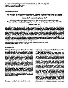
construct a general index of the stringency of environmental policy regimes. A number of imperfect proxies have been used in empirical work. This includes reported data on pollution abatement and control expenditure measured at the macroeconomic (e.g., Lanjouw and Mody 1996) or sectoral level (e.g., Brunnermeier and Cohen 2003), the frequency of inspection visits (e.g., Jaffe and Palmer 1997), parameterisation of policy types (e.g., Fischer and Newell 2008, Johnstone 2007). One of the few studies to use commensurable measures of actual policy stringency across countries is Johnstone et al. (2010), but this relates to only one sector (renewable energy). This study draws upon data obtained from the World Economic Forum’s “Executive Opinion Survey”, which asked respondents a number of questions related to environmental policy design. The survey was implemented by the WEF’s partner institutes in over 100 countries, which include departments of economics at leading universities and research departments of business associations. The means of survey implementation varied by country and included postal, telephone, internet and face-to-face survey. In most years, there were responses from between 8,000 and 10,000 firms (see WEF 2008 for a description of the sampling strategy.) In the WEF survey, respondents (usually CEOs) were requested to indicate the “stringency” of a country’s overall environmental regulation. More specifically, they were requested to assess the degree of stringency on a Likert scale, with 1 = lax compared with that of most other countries, 7 = among the world’s most stringent. The variable ranges from 1.4 (Haiti) as its lowest to 6.7 (Germany) as its highest value in our sample. The index varies slightly over the seven years considered in our analysis. In Figure 1 the measure of stringency of environmental policy of the source country is plotted against the log of total outgoing FDI flows relative to source country’s gross domestic product. We use mean values for the period 2001-2007. Stringency of the source country (all source countries in the sample are members of the OECD) appears to have a clear and seemingly strong positive impact on the outgoing investment flows, providing descriptive evidence to support the pollution haven hypothesis.

-17

Figure 1. Environmental regulation stringency of the source country (OECD members) and outgoing FDI flows (relative to GDP of the source country), based on average values (2001-2007)

log(total FDI outflow to source GDP) -21 -20 -19 -18

NOR AUT CHE NLD ESP HUN

BEL SWE

ISL GBR

KOR FRA

FIN

DNK DEU

POL CZE

NZL USA JPN AUS

GRC

IRL SVK

-22

ITA

TUR

3

4

5 6 Stringency of the source country

8

7

In Figure 2 a scatter plot of the stringency of the host country and inward FDI (the log of total incoming flows relative to the host country’s gross domestic product) is presented. The results are presented for both OECD and non-OECD host countries. Not surprisingly, the majority of the OECD sample lies in the right half of the graph and vice versa for the developing countries. While the effect in the OECD sample is not clear, the relationship between stringency and FDI in the developing countries seems to be somewhat positive. There are two possible explanations for the last observation. First, stringency of environmental regulation may be catching the potential effect of the quality of institutions in the developing countries. The correlation coefficient between environmental stringency and regulatory quality in our sample is equal to 0.75. It is widely known in the literature that better quality of institutions attracts more FDI inflows, and therefore the apparent positive relationship may be explained by this relationship. In order to get the “clean” correlation between stringency and FDI in the host country we have to control explicitly for its regulatory quality in our empirical analysis. Second, the relationship between stringency and FDI may be non-linear, as predicted in the hypothesis, but Figure 2 does not account for that.

-14

Figure 2. Environmental regulation stringency of the host country and incoming FDI flows (relative to GDP of the host country), based on average values (2001-2007)

log(total FDI inflow to host GDP) -20 -18 -16

NLD

PAN

MUS

EST

HUN IRL SGP

CHE BEL SVK HRV HKG GBR UKR GHA NZL FIN AUT KAZ LTU PRT CAN POL CZE ZAF SWE RUS ESP CRI SLV NOR SVN MDG VNM MEX CHL AUS MYS THA TUR NGA MAR BWA DEU FRA DNK PER TUN ITA ARE ZWE KEN EGY URY BRA DZA GRC VEN CMR IDN ISR LVA MOZ DOM MWI TCD ECU HND ARG MKD SEN ZMB SEN BHR KOR USA CHN BOL BIH BIHPAK PAK IND COL JOR NAM PHL TZA LKA ROM BGR

HTI

ETH GTM

GMB

JPN

MLI

-22

BGD

0

2

ISL

4 Stringency of the host country

6

8

And finally, Figure 3 plots the difference in environmental stringency between the source and host countries against bilateral FDI flows (relative to source country’s GDP). OECD source countries are identified in the graph with triangles, and non-OECD host countries with circles. It becomes evident that the OECD host countries are predominantly situated in the left part of the figure where the values for the difference variable are negative (i.e. environmental regulation in the source country is less stringent than the one in the host country) or rather low positive (i.e. source and host countries have a similar level of environmental stringency). No discernible pattern is evident within each group of countries. However, since there are so many factors which are likely to influence FDI, the absence of an obvious pattern in the bivariate relationship is hardly surprising.

9

-35

log(FDI outflow to source GDP) -30 -25 -20 -15

Figure 3. Difference in environmental regulation stringency between source and host country and outgoing FDI flows (relative to GDP of the source country), average values (2001-2007)

-4

-2 0 2 4 Difference in stringency between source and host country OECD host countries

6

non-OECD host countries

3. Empirical results 3.1. Baseline results In the baseline specification, we regress the (natural) logarithm of outbound FDI flows on the environmental stringency gap between the source and host countries, controlling for all KC variables. The baseline results are presented in Table 1. Column (2) considers the whole sample, namely OECD countries investing into the OECD and non-OECD world. Since combining rich and poor countries in FDI data can lead to implausible coefficient estimates, column (3) reports only OECD investment into the non-OECD world, while capital transactions in the OECD region can be found in column (4). Despite the skewed nature of the dependent variable, many studies, including Carr et al. (2001, 2003), Markusen and Maskus (2002) and Davies (2008), use the absolute value of FDI instead of its logarithmic value. To check our findings against this part of the literature we report in column (1) the Tobit results for the whole sample with the absolute value of FDI flows as the dependent variable. To account for potential interdependencies between the bilateral FDI flows into a host country and from a certain source country, we report only heteroskedasticity-robust standard errors. In Table A-2 in the appendix we present descriptive summary statistics for the whole sample. Summarizing, the analysis provides strong and consistent support for the main hypothesis, according to which a larger positive stringency differential increases FDI flows from the source to the host country. Furthermore, an inverse U-shape relationship between the stringency differential and FDI exists in the OECD to non-OECD sample.

10

Table 1. Main results: panel estimation for the period 2001-2007 Tobit estimation Variables

OECD to Whole sample

non-OECD OECD only (1) (2) (3) (4) Sum of GDP 3.19E-09*** 6.52E-13*** 1.34E-12*** 1.07E-13 (5.90E-10) (2.20E-13) (3.96E-13) (2.90E-13) GDP difference -7.53E-23*** -2.93E-26*** -4.25E-26** -2.18E-26*** squared (1.84E-23) (6.56E-27) (1.81E-26) (7.58E-27) Interaction term I 1.63E-15 -3.15E-18 -8.28E-18*** -1.53E-18 (2.75E-15) (2.34E-18) (2.84E-18) (2.72E-18) Interaction term II -1.64E-14*** 1.81E-18 9.39E-18*** 5.64E-19 (3.84E-15) (2.35E-18) (3.07E-18) (2.81E-18) Interaction term III -8.81E-15** 2.48E-18 -5.45E-17 2.26E-18 (3.83E-15) (1.73E-18) (4.40E-17) (1.89E-18) Distance -0.1799556*** -0.0002292*** -0.0002916*** -0.0001842*** (0.0223926) (0.000016) (0.0000197) (0.0000296) Customs union 419.5397** 0.6894951*** 0.6155521** 1.224973*** (204.3149) (0.1885257) (0.2828086) (0.3755362) Free trade agreement 122.7988 0.4805627*** 0.6560606*** 0.7275514** (180.0684) (0.1625127) (0.1900295) (0.3658471) Common border 1400.38*** 1.412304*** 2.778845*** 1.440371*** (205.456) (0.1639131) (0.2404604) (0.2007996) Common language 1374.476*** 1.121314*** 2.230499*** 0.4175423 (247.4375) (0.1724089) (0.2142102) (0.2691453) Regulatory quality -104.0356 0.5393671** 0.7347263** 0.3073314 (273.0012) (0.2673918) (0.2962141) (0.5165112) Stringency difference -36.15144 -0.0189284 0.3414885** 0.0666871 (102.9803) (0.0939953) (0.1358803) (0.1432315) Stringency difference 58.96386*** 0.0336511** -0.0824404*** 0.0496366* squared (19.55608) (0.0148894) (0.025334) (0.0267563) Intercept -3366.931*** 0.531365 -0.6881165 7.406962** (801.8365) (0.7072599) (0.769801) (3.230629) Observations 9711 9711 5071 4640 Uncensored obs. 5822 5822 2673 3149 (Pseudo) R-squared 0.03 0.17 0.21 0.12 Notes: i) *** - significant at 1% level, ** - significant at 5% level, * - significant at 10% level; ii) Robust standard errors in parentheses; iii) The dependent variable in column (1) is the level of FDI, while columns (2)-(4) explain the natural logarithm of FDI; iv) All columns present Tobit estimates; v) All estimations include year, source and host country fixed effects.

To assess our main hypothesis, we consider the joint effect of the two stringency variables: ∆𝑆𝑡𝑟𝑖𝑛𝑔𝑒𝑛𝑐𝑦 and (∆𝑆𝑡𝑟𝑖𝑛𝑔𝑒𝑛𝑐𝑦)2. Let us look first at the results for the whole sample. The predicted positive effect of an increasing stringency gap on FDI is clearly supported in columns (1) and (2). Although only the squared term of stringency enters with a significant sign, it is strongly positive. The magnitude of the effect differs along the two columns, because of regressing FDI in levels and its natural logarithm in column (1) and (2), respectively.

11

In a next step, we look at the sample of OECD countries investing in non-OECD countries. Column (3) clearly shows that the stringency gap between the OECD source and the non-OECD host country has a positive effect on FDI. Furthermore, there is evidence of an inverse U-shaped relationship, since the squared term enters with a negative sign. This result is highly relevant for the policy discussion, where OECD governments fear that their industries move to less developed countries with laxer environmental standards. This is truly the case as our results suggest, however only up to a certain threshold. Once the difference in stringency between the source and the host country has reached a value of 2.1 6, the effect on FDI is reversed (see Figure 4). Thus, once the environmental regime of a host country becomes too lax, this country loses its attractiveness as an FDI location. In Figure 4 we simulate the effect of the stringency gap on FDI in the non-OECD sample. Brazil, Costa Rica, Singapore and Hong Kong are some of the non-OECD host countries which have rather low stringency gaps with the developed OECD area and thus lie to the left of the threshold value of 2.1. This evidence implies that a further strengthening of the environmental regimes in these countries would make them less attractive for FDI flows. In contrast, to the right of the threshold values we can find countries like Croatia, Egypt, Morocco, Russia, Venezuela, which are characterized by large stringency gaps with the OECD world. For this group of countries a further weakening of their already lax environmental policies would deteriorate their investment climate and thus lead to a decrease in FDI inflows. A potential explanation for this result is that stringency of environmental regulation is often positively related with policy predictability, and may account partly for the latter. As such a low level of stringency would be equivalent to a confusing and frequently changing environmental regime. 7 Consequently, policy unpredictability may be associated with corruption and fear of expropriation. In technical terms, we face an omitted variable problem, which might be solved by accounting separately for stringency and predictability. Due to the high correlation between these two policy attributes, however, such an empirical exercise will be fundamentally flawed. Last, we discuss the within-OECD investment activity (column 4). The results confirm those in columns (1) and (2), where we find a clear positive impact of the environmental stringency gap on FDI flows. This is not surprising, because most of the non-zero investment flows are observed for this sample, which then may drive the result of the whole sample. The positive and significant sign for the main explanatory variable, the stringency difference, implies a “pollution-haven” effect in the OECD area itself. It is an important result for policy makers who very often refer to the developing world concerning lax environmental regulations. Indeed the OECD countries do not form a homogenous group in terms of environmental stringency, at least in so far as perceived by the business community.

6

We calculate the number by using the estimated coefficients in column (3): 2.1=0.34/2*0.08. The correlation between the policy stringency variable, and another variable reflecting the “clarity and stability” of environmental policy is over 0.85.

7

12

Figure 4. Estimates for the sample of non-OECD host countries logFDI average values

panel estimation

-2.9

-2.5

-2

-1.5

-1

-0.5

0

0.5

1

1.5

2

2.5

3

3.5

4

4.5

5

5.4

Stringency differential

We can also look briefly at the other controls in the baseline model. The sum of a host country’s and a source country’s GDP affects investment positively. We find that FDI is strictly decreasing in the squared GDP difference. These qualitative results are in line with the KC model predictions of a U-shaped relationship between the FDI flow and bilateral differences in economic size. The three interaction terms allow us to make conclusions about the mode of production fragmentation among the countries in the three different samples. Since Interaction terms II and III enter with a negative sign, while Interaction term I is insignificant in column (1), horizontal investment seems to be the predominant model of FDI activity across the whole sample. This result, however, changes when we consider the non-OECD host countries only. The negative sign for the coefficients of Interaction term I and III and the positive sign for the second term predict vertical FDI. Common evidence suggests that the majority of FDI from the developed world to developing countries flows into production facilities because of the difference in factor endowments between the source and host country. In contrast, the three interaction terms do not have a clear-cut effect on FDI in the OECD sample (column 4), which restrains us from making conclusions about the predominant FDI model there. Distance has a consistent negative estimate across our results. The four proxies for bilateral trade costs have a very strong positive impact often at the 1% significance level across the different samples, as expected. The positive and mostly significant sign in front of the regulatory quality variable, our proxy for costs associated with setting up a business, is in line with the theoretical predictions. In conclusion, while the fundamentals of the KC model remain important determinants of FDI flows, the stringency gap proves to be a powerful explanatory factor as well. The findings are robust with respect to a number of alternative specifications 8. 3.2. Estimates using averages Since our measure of environmental stringency varies only slightly over time, estimating a panel may be regarded as an unjustified inflation of the sample size, besides controlling for fixed country effects. For this reason, the model was also estimated by using average values (see Table 2). We therefore collapse all variables to their 2001–2007 averages. The results of this estimation clearly support and reinforce our findings from the panel fixed effects regressions in Table 1. 8

In the next sub-section we estimate the model with average values. Furthermore, we run a number of robustness checks by using alternative explanatory variables, accounting for additional regressors such as tariffs and corporate income taxes, as well as dropping host country outliers with very low and very high stringency levels. The sensitivity analysis clearly confirms our main results and is available upon request.

13

Column (2) confirms the inverse U-relationship between stringency and FDI in the sample of non-OECD host countries. The threshold value lies at 2.9 (=0.4053677/(2*0.0458561)), which implies that once the difference in the levels of stringency between the source and host country increases beyond this value, FDI will be decreasing (see Figure 4). In contrast, column (3) indicates a significant and persistent positive relationship between FDI and stringency among OECD countries. The result suggests that “pollution havens” may exist rather in the fellow OECD countries and the progressive emerging economies than in the low-income and unskilled-labour abundant developing countries. For the whole sample, in column (1) the stringency difference and its squared term are significant and with the expected signs. However, the calculations do not provide a clear evidence of a hump-shape relationship between stringency and FDI, since the optimal value for the stringency gap lies nearly out-of-sample (4.4=0.4053677/2*0.0458561) 9. Table 2. Results with average values Dependent variable: logFDI_ij Variables Sum of GDP GDP difference squared Interaction term I Interaction term II Interaction term III Distance Customs union Free trade agreement Common border Common language Regulatory quality Stringency difference Stringency difference squared Intercept Observations

Whole sample (1) 1.42E-12*** (1.22E-13) -1.16E-25*** (1.16E-26) -2.48E-17*** (5.72E-18) 2.78E-17*** (5.99E-18) 2.17E-18 (3.69E-18) -0.0002173*** (0.0000191) 0.2463042 (0.2045682) -0.0652349 (0.1738802) 1.957943*** (0.2883588) 1.194777*** (0.2500466) 1.385794*** (0.1196797) 0.4053677*** (0.072174) -0.0458561** (0.0204392) 0.1234822 (0.2151097) 2436

9

OECD to non-OECD (2) 2.14E-12*** (1.65E-13) -1.5E-25*** (1.33E-26) -3.46E-17*** (5.64E-18) 2.66E-17*** (7.14E-18) 1.30E-16 (9.16E-17) -0.0001942*** (0.000023) -0.2131343 (0.3233686) 0.4989409** (0.2258893) 3.093692*** (0.5304518) 1.088267*** (0.2788683) 1.010685*** (0.1463677) 0.6865922*** (0.1581523) -0.1190785*** (0.0377199) -0.6416254** (0.2502088) 1689

OECD only (3) 9.66E-13*** (1.06E-13) -6.67E-26*** (1.25E-26) -3.95E-18 (4.65E-18) 9.18E-18 (6.05E-18) -1.11E-18 (3.71E-18) -0.0002478*** (0.0000324) -0.1118559 (0.3149657) -0.6468675** (0.2815686) 1.629879*** (0.3696259) 1.664561*** (0.4967006) 1.855155*** (0.3622611) 0.6399197*** (0.106928) 0.0998556* (0.054118) 0.5819667 (0.7107843) 747

Only the stringency difference between the ten OECD countries with the most stringent environmental regimes in our sample and four developing countries – Angola, Ethiopia, Haiti and Macedonia – goes beyond this threshold value.

14

Uncensored obs. 1443 858 585 (Pseudo) R-squared 0.13 0.12 0.09 Notes: i) *** - significant at 1% level, ** - significant at 5% level, * - significant at 10% level; ii) Robust standard errors in parentheses, iii) All columns present Tobit estimates.

3.3. Quantitative importance The estimated coefficients presented above can be interpreted quantitatively, by calculating their marginal effects at the sample means of the covariates. Furthermore, the calculations take into account the nonlinear function of the stringency differential. We consider only the baseline panel estimation results (Table 1) and begin with the whole sample, first. The marginal effect of the stringency gap is equal to 0.027 in the whole sample. It then becomes easy to calculate that a one-unit increase in ∆Stringency is associated with a 2.7% (=100*[exp(0.027)-1]) increase in the FDI flow. As part of the total marginal effect 1.9% is the effect of stringency on investment within the sample of country pairs that are already experiencing positive FDI flows. Column (1) of Table (1) reinforces the positive impact of the stringency variable. However, the results are interpretable in a different way, since the dependent variable is in levels. The marginal effect is calculated to be 24.41, which means that only one unit increase in the stringency gap suffices for an increase of outward FDI by 24 Million US dollars. The sample of the non-OECD host countries yields similar results. However, the effect of the difference in the stringency levels between the source and host country are higher than in the whole sample. The total marginal effect of 0.038 translates into 4% increase in FDI, while country pairs that are already investing partners experience 2.7% increase in FDI for a one-point increase in the stringency gap. The strongest effect of environmental stringency on FDI activity is observed, however, in the OECD sample, where FDI flow increases by 5.5% if the stringency gap rises by one unit, and by 4% in the positive FDI sample. What is the relative magnitude of the environmental stringency in comparison to other explanatory factors, such as regulatory quality and common border? The large estimates of these two variables in Table 1 translate also into large marginal effects. Thus, a one-unit improvement of regulatory quality brings 44% increase in FDI in the whole sample and 54% increase, when OECD countries invest to nonOECD host countries. Governance quality seems to be less relevant, when investing in a fellow OECD country. This outcome indirectly suggests the high importance of regulatory quality as a signal, in particular, about countries that do not belong to a well-known "league". Sharing a common border between an OECD source and non-OECD host country will bring an estimated 400% increase in FDI flows to the host. The effect is lower but still significantly large in the OECD sample, at around 200%. The economic and geographic fundamentals of the KC model play a very important role in foreign investment decisions. In comparison, the rather low magnitude of the effect of environmental stringency appears plausible and gives an indication of the size of the potential loss from policy stringency on the investment climate. 4. Conclusion This paper provides new evidence on the ‘pollution haven effect’. Using ‘state of the art’ methodology, a new measure or environmental policy stringency, and a very broad sample, support is found for the effect of relative environmental policy stringency on foreign direct investment patterns. Pollution havens are shown to exist not only in the developing world but also in the OECD area itself. This is an important result for the policy discussion, which has generally focussed on the differences in environmental regulation between developed and developing countries and thus neglected the heterogeneity in the group of the OECD countries. However, it must be emphasised that the effect of environmental stringency is 15

relatively small in comparison with other factors such as regulatory quality and trade costs. Moreover, the relationship appears to be non-linear with the effects of increased relative environmental policy stringency in the non-OECD host country decreasing (and becoming negative) after a certain threshold. This non-linear relationship may be due to a combination of three factors. First, above a certain level, increased stringency increases production costs and reduces the attractiveness of the country for foreign investors. Second, for investment flows from OECD to non-OECD countries there is a certain level which is more or less costless, perhaps due to economies of standardisation across different production locations. Finally, below this level, there may be a ‘signalling’ role played by environmental policy, with excessively lax policy indicating a more uncertain (and thus less attractive) environment for investment. In this vein, is important to bear in mind that the measure of environmental policy stringency used in this analysis is based on subjective perceptions of the business community, and is not an objective measure. However, for the reasons mentioned above, results based upon a subjective measure may be more policyrelevant. Decisions concerning foreign direct investment are necessarily based on imperfect information. If our measure of environmental policy stringency ‘signals’ broader regulatory quality to investors then the finding that a sufficient gap between source and host country policy stringency has a negative effect on FDI flows is not surprising and supports findings elsewhere in the literature. This is also reassuring insofar as it indicates that there is a limit to the ‘chilling’ effect, which could serve as a disincentive to introduce optimally stringent environmental policy and/or an incentive to introduce protectionist trade or investment policies. Beyond this, the policy implications of the results for OECD countries are two-fold: •

There is a strong case to be made for capacity-building with respect to the environmental policy framework in non-OECD countries since this can yield both environmental and economic benefits to host countries. With long experience in policy implementation and assessment OECD countries can play an important role in facilitating this capacity building; and,

•

Since there is evidence of the impact of policy stringency on FDI amongst OECD countries international cooperation in the development of policy measures may yield benefits. This is particularly the case for transfrontier pollutants, since ‘leakage’ will undermine the attainment of domestic environmental objectives. However, it must be emphasised that the effect of environmental policy stringency on FDI (and thus leakage) is small.

16

APPENDIX Table A-1. Data sources Variables

Description

FDI

Flow of foreign direct investment from the source to the host country; Source: OECD International Direct Investment Statistics Yearbook. Difference / Sum of gross domestic products between source and host country in US dollars with base year 2000; Source: World Development Indicators (WDI). Difference of GDP per capita between source and host countries in number of years; in the sensitivity analysis we also use the difference of education duration; Source: WDI. Interaction term equal to ∆𝑆𝑘𝑖𝑙𝑙 ∗ ∆𝐺𝐷𝑃 if ∆𝑆𝑘𝑖𝑙𝑙 > 0, and 0 otherwise. Interaction term equal to ∆𝑆𝑘𝑖𝑙𝑙 ∗ ∑ 𝐺𝐷𝑃 if ∆𝑆𝑘𝑖𝑙𝑙 > 0, 0 otherwise. Interaction term equal to −∆𝑆𝑘𝑖𝑙𝑙 ∗ ∑ 𝐺𝐷𝑃 if ∆𝑆𝑘𝑖𝑙𝑙 < 0, 0 otherwise. Distance in km between the capitals of the source and host country; Source: Centre d’Etudes Prospectives et d’Informations Internationales (CEPII). A binary variable equal to 1 if the source and host country share the same language and 0 otherwise; Source: CEPII. A binary variable equal to 1 if the source and host country share the same border and 0 otherwise; Source: CEPII. A binary variable equal to 1 if the source and host countries belong to the same customs union and 0 otherwise; Source: World Trade Organization (WTO), own compilation. A binary variable equal to 1 if the source and host countries belong to the same free trade agreement and 0 otherwise; Source: WTO, own compilation. Rating of regulatory quality in host country with a range from -2.5 to 2.5; Source: Kaufmann et al. (2008). Difference of the stringency levels of environmental regulation between the source and host country; Source: World Economic Forum.

ΣGDP, ∆GDP ∆Skill Interaction term I Interaction term II Interaction term III Distance Common Language Common Border Customs Union Free Trade Agreement Regulatory quality ∆ Environmental Stringency

Table A-2. Descriptive statistics for the whole sample, 9711 observations Variable

Standard Deviation

Mean

Minimum

Maximum

LogFDI

2.517635

2.841828

0

11.57918

Sum of GDP

1.66E+12

2.71E+12

1.48E+10

1.67E+13

GDP difference squared

8.06E+24

2.57E+25

1.60E+15

1.31E+26

Interaction term I

1.78E+16

6.60E+16

-4.16E+17

4.98E+17

Interaction term II

2.65E+16

6.76E+16

0

5.96E+17

Interaction term III

6.61E+15

2.91E+16

0

4.35E+17

Distance

6081.383

4907.198

59.61723

19629.5

Customs union

0.2241788

0.4170618

0

1

Free trade agreement

0.2140871

0.4102087

0

1

Common border

0.0510761

0.2201643

0

1

Common language

0.0679642

0.2516974

0

1

Regulatory quality

0.7015062

0.8633914

-2.173003

2.011307

Stringency difference

0.880589

1.529691

-3.9

5.4

Stringency difference squared

3.115152

3.803315

0

29.16

17

REFERENCES Alfaro, L. and A. Charlton (2009). “Intra-Industry Foreign Direct Investment”, American Economic Review, 99, 2096-2119. Ambec S. and P. Barla (2002). “A theoretical foundation of the Porter hypothesis”, Economics Letters, 75, 355-360. Ambec, S. and Barla P. (2007). ”Quand la réglementation environnementale profite aux pollueurs. Survol des fondements théoriques de l'hypothèse de Porter”, L’Actualité économique, 83(3), 399-414. Blonigen, B.A., R.B. Davies and K. Head (2003). “Estimating the Knowledge-Capital Model of the Multinational Enterprise: Comment”, American Economic Review, 93, 980-994. Brunnermeier, S.B. and M.A. Cohen (2003). “Determinants of environmental innovation in US manufacturing industries”, Journal of Environmental Economics and Management, 45, 278-293. Brunnermeier, S. and Levinson, A. (2004). Examining the evidence on environmental regulations and industry location, Journal of Environment and Development, 13, 6–41. Carr, D.L., J.R. Markusen, and K.E. Maskus (2001). “Estimating the Knowledge-Capital Model of the Multinational Enterprise”, American Economic Review, 91, 693-708. Carr, D.L., J.R. Markusen, and K.E. Maskus (2003). “Estimating the Knowledge-Capital Model of the Multinational Enterprise: Reply”, American Economic Review, 93, 995-1001. Constantini, V. and M. Mazzanti (2010). “On the green side of trade competitiveness? Environmental policies and innovation in the EU”, Fondazione Eni Enrico Mattei Working Paper No 2010.94. Copeland, B.R. and M.S. Taylor (2004), “Trade, Growth and the Environment.” Journal of Economic Literature, 42, 7-71. Davies, R.B. (2008). “Hunting High and Low for Vertical FDI”, Review of International Economics, 16, 250-267. Ederington, J. and J. Minier (2003). “Is Environmental Policy a Secondary Trade Barrier? An Empirical Analysis”, Canadian Journal of Economics, 36, 137-154. Eskeland, G.S. and A.E. Harrison (2003). “Moving to Greener Pastures? Multinationals and the Pollution Haven Hypothesis”, Journal of Development Economics, 70, 1-23. Fischer C. and R.G. Newell (2008). “Environmental and technology policies for climate mitigation”, Journal of Environmental Economics and Management, 55, 142-162. Gabel, H.L. and B. Sinclair-Desgagné (2002). “The firm, its procedures, and win-win environmental regulations” in: Henk Folmer et al. Frontiers of Environmental Economics (Cheltenham, UK). Helpman, E. (1984). “A Simple Theory of International Trade with Multinational Corporations”, Journal of Political Economy, 92, 451-471.

18

Henderson, D.J. and D.L. Millimet (2007). “Pollution Abatement Costs and Foreign Direct Investment Inflows to U.S. States: A Nonparametric Reassessment”, Review of Economics and Statistics, 89, 178-183. Jaffe, A.B.; R.G. Newell, and R.N. Stavins (2005). "A tale of two market failures: Technology and environmental policy," Ecological Economics, 54, 164-174. Jaffe, A. B. and K. Palmer (1997), “Environmental regulation and innovation: A panel data study”, The Review of Economics and Statistics, 79, 610-619. Jeppesen, T., J.A. List, and H. Folmer (2002). “Environmental Regulations and New Plant Location Decisions: Evidence from a Meta-Analysis”, Journal of Regional Science, 42, 19-49. Johnstone, N. (2007). Environmental Policy and Corporate Behaviour (Cheltenham, UK: Edward Elgar). Johnstone N., Hascic I., and D. Popp (2010). “Renewable energy policies and technological innovation: Evidence based on patent counts”, Environmental and Resource Economics, 45, 133-155. Keller, W. and A. Levinson (2002). “Pollution Abatement Costs and Foreign Direct Investment Inflows to US States”, Review of Economics and Statistics, 84, 691-703. Kennedy, P. (1994). “Innovation stochastique et coût de la réglementation environnementale,” L’Actualité économique, 70, 199-209. Kessing, S.G., K.A. Konrad, and C. Kotsogiannis (2009). “Federalism, Weak Institutions and the Competition for Foreign Direct Investment”, International Tax and Public Finance, 16, 105-123. Lanjouw, J.O. and A. Mody (1996), “Innovation and the international diffusion of environmentally responsive technology”, Research Policy, 25, 49-571. Lanoie, P., M. Patry, and R. Lajeunesse (2008). “Environmental Regulation and Productivity: Testing the Porter Hypothesis”, Journal of Productivity Analysis, 30, 121-128. Levinson, A. (1996). “Environmental Regulations and Manufacturers’Location Choices: Evidence from the Census of Manufacturers”, Journal of Public Economics, 62, 5-29. Levinson, A. and M.S. Taylor (2008). “Unmasking the Pollution Haven Effect”, International Economic Review, 49, 223-254. Li, Q. (2009). “Democracy, Autocracy, and Expropriation of Foreign Direct Investment”, Comparative Political Studies, 42, 1098-1127. List, J.A. and C.Y. Co (2000). “The Effects of Environmental Regulations on Foreign Direct Investment”, Journal of Environmental Economics and Management, 40, 1-20. Markusen, J.R. (1984). “Multinationals, Multi-Plant Economies, and the Gains from Trade”, Journal of International Economics, 16, 205-226. Markusen, J.R. and K.E. Maskus (2002). “Discriminating among Alternative Theories of the Multinational Enterprise”, Review of International Economics, 10, 694-707.

19

Millimet, D.L. and J.A. List (2004). “The Case of the Missing Pollution Haven Hypothesis”, Journal of Regulatory Economics, 26, 239-262. Mohr R.D. (2002). “Technical change, external economies, and the Porter hypothesis”, Journal of Environmental Economics and Management, 43, 158-168. Oates, E.; K. Palmer, and P.R. Portney (1995). “Tightening environmental standards: the benefit-cost or the no-cost paradigm?”, Journal of Economic Perspectives, 9(4) 119-112. Organisation for Economic Co-Operation and Development (2009). “Linkages between Environmental Policy and Competitiveness”, ENV/EPOC/GSP(2008)14/FINAL. Porter, M. and C. van der Linde (1995). “Towards a new conception of environment-competitiveness relationship”, Journal of Economic Perspectives, 9, 97-118. Simpson, D. and R.L. Bradford (1996). “Taxing variable cost: environmental regulation as industrial policy”, Journal of Environmental Economics and Management, 30(3), 282-300. Smarzynska Javorcik, B. and S.-J. Wei (2005). "Pollution Havens and Foreign Direct Investment: Dirty Secret or Popular Myth?", The B.E. Journal of Economic Analysis & Policy, Berkeley Electronic Press, vol. 0(2). Taylor, M.S. (2004). “Unbundling the pollution haven hypothesis”, Advances in Economic Analysis and Policy, 4, Article 8. Wagner, U.J. and C.D. Timmins (2009). “Agglomeration Effects in Foreign Direct Investment and the Pollution Haven Hypothesis”, Environmental and Resource Economics, 43, 231-256. Waldkirch, U. and M. Gopinath (2008). “Pollution Control and Foreign Direct Investment in Mexico: An Industry Level Analysis”, Environmental and Resource Economics, 41, 289-313. World Economic Forum (2008), The Global Competitiveness Report (Oxford University Press, New York). Wheeler (2001). “Racing to the Bottom? Foreign Investment and Air Pollution in Developing Countries”, Journal of Environment and Development, 10, 225-245. Xing, Y. and C. Kolstad (2002). "Do Lax Environmental Regulations Attract Foreign Investment?," Environmental and Resource Economics, 21(1), 1-22.

20