Effects of curve number modification on runoff estimation using WSR-88D rainfall data in Texas watersheds J.H. Jacobs and R. Srinivasan ABSTRACT: The purpose of this study was to evaluate variations of the Natural Resources Conservation Service (NRCS) curve number method for estimating near real-time runoff for naturalized flow, using high resolution radar rainfall data in Texas watersheds. This study was undertaken in an attempt to provide more accurate runoff estimates to watershed and water resource managers for planning purposes. Stage III Weather Surveillance Radar 1988 Doppler (WSR-88D) precipitation data, obtained from the West Gulf River Forecast Center, was used as the precipitation input for runoff estimates in this study. The study areas consisted of dominant or homogenous land use and were characterized by naturalized flow. Findings indicate that the use of a dry antecedent soil moisture condition curve number value and a reduced initial abstraction coefficient (Ia ) in the NRCS curve number equation produced the most statistically significant comparison between observed and estimated runoff in nine out of ten watersheds. The combined comparison for all events in these nine watersheds produced a coefficient of efficiency (COE) of 0.70, with a slope of 0.78 and an r2 of 0.77. Overall, the results of this research suggest that, although further improvements can be made for improved runoff estimation, the use of modified inputs to the NRCS curve number equation in conjunction with WSR-88D radar rainfall data could be useful in producing runoff estimates for Texas in real-time. Keywords: Hydrologic modeling
Water availability has become a major issue in Texas in recent years. Adding to this issue is the expected doubling of the population within the next 50 years, mainly in areas presently without abundant water supplies. To combat problems that Texas will face in the future, there has been a move toward active planning and management of water resources. Real-time weather data processing and hydrologic modeling can provide information for this planning in addition to flood and drought mitigation, reservoir operation, and watershed and water resource management practices (Texas Water Development Board, 2000). However, in order to provide this information to managers, it is necessary to first obtain reliable and readilyavailable weather data. Rain gauge networks are generally sparse and insufficient to capture the spatial variability of rainfall across large watersheds, especially
274
JOURNAL OF SOIL AND WATER CONSERVATION S| O 2005
in arid and semi-arid regions, such as west Texas, where most rainfall occurs in short, heavy, localized thunderstorms. Dense networks necessary to provide such data are generally available only for experimental or research watersheds. Also, few rain gauge networks are currently able to provide realtime data. The use of weather radar systems could help alleviate these problems. One such system is the Weather Surveillance Radar 1998 Doppler (WSR-88D) of the National Weather Service (NWS). This data could be used in conjunction with runoff models, such as the Natural Resources Conservation Service (NRCS) curve number method to deliver data to managers in a near real-time fashion. In the 1950’s, the curve number method was developed to estimate runoff in ungauged watersheds (SCS, 1972). This method is widely used for watershed model-
ing, and has been incorporated into various computer models worldwide (Woodward et al., 2002; Hawkins et al., 2002). Although this is an accepted method for runoff estimation, studies have indicated that it should be evaluated and adapted to regional agroclimatic conditions. Hawkins (1998) states that curve number tables should be used as guidelines and that actual curve numbers and their empirical relationships should be determined based on local and regional data. This is supported by Van Mullem et al. (2002). They state that the direct runoff calculated by the curve number method is more sensitive to the curve number variable than rainfall inputs. This would suggest an increased need for field verification of land cover type and condition before curve number assignment. The accuracy of hydrologic models depends on the accuracy of input data and, in the case of the NRCS curve number method, the variable inputs. The purpose of this study was to evaluate several variations of the NRCS curve number method for estimating near real-time runoff for naturalized flow, using WSR-88D rainfall data for watersheds in various agro-climatic regions of Texas in an attempt to represent the spatial variability of rainfall. Methods and Materials Study area selection and description. Ten watersheds of varying size (355 to 2,940 km2), in four river basins, throughout different agro-climatic regions of Texas were used in this study to account for a variety of hydrologic conditions throughout the state (Figure 1). Watersheds were chosen based on dominant land use, soil hydrologic group, and streamgauge location (Table 1). Land cover data was obtained from the 1992 U.S. Geological Survey (USGS) National Land Cover Dataset at a 1:24,000 scale (30 m resolution). Only watersheds with homogenous/dominant cover or similar curve number values were used. Soils data were derived from the U.S. Department of Agriculture Natural Resources Conservation Service (USDA-NRCS) State Soil Geographic (STATSGO) database, at a 1:250,000 scale (250 m resolution). Streamflow data was Jennifer H. Jacobs is a research associate and Raghavan Srinivasan is the professor and director at the Spatial Sciences Laboratory at Texas A&M University in College Station, Texas.
Reprinted from the Journal of Soil and Water Conservation Volume 60, Number 5 Copyright © 2005 Soil and Water Conservation Society
Figure 1 Study area locations.
(3) For the actual runoff calculation, initial abstractions (Ia) are generally approximated as 0.2 retention parameter, and the basic equation becomes (Equation 4):
Red-1
Red-2 Trinity-1
(4)
LCR-1
Trinity-2
where, Qsurf = surface runoff in mm, Rday = rainfall depth for the day, also in mm.
Trinity-3
LCR-2 LCR-3 SA-1
SA-2 N
W
0
50
100
200 Kilometers
downloaded from the USGS website for each watershed outlet. Total streamflow is composed of baseflow (lateral flow and shallow ground water discharge to streams) and surface runoff. To compare measured flow and estimated runoff (NRCS curve number method provides only direct runoff after a rainfall event), it was necessary to determine the portion of streamflow that could be attributed to surface runoff. Therefore, flow data was processed through a filter program. The filter program developed by Arnold et al. (1995) was used in this study, and is comparable to other automated separation techniques, with 74 percent efficiency when compared to manual separation (Arnold and Allen, 1999). Also, because the runoff algorithms used in this study do not account for reservoirs or other diversions, only sites with natural, or unregulated, flow were used. This allowed for a direct comparison of runoff estimates to measured streamflow data. Curve number calculations. Daily runoff calculations were generated using the NRCS curve number method. This calculation is based on the retention parameter, S, initial abstractions, Ia (surface storage, interception, and infiltration prior to runoff), and daily rainfall, Rday, (all in mm H20). The retention parameter is variable due to changes in soil type, land use, and soil moisture, and is
E
S
defined as (Equation 1):
(1)
Curve number varies based on one of three antecedent soil moisture conditions, curve number I-dry (wilting point), curve number II-average, and curve number III-wet (field capacity) (Neitsch et al., 2001). Runoff estimates increase with increasing antecedent soil moisture condition, and with increasing curve number. Curve number II was assigned based on the dominant land use from National Land Cover Dataset and soil hydrologic group from STATSGO according to the Soil Conservation Service’s (SCS) Texas Engineering Technical Note No. 210-18-TX5 (1990). Curve number I and curve number III are calculated from curve number II and are defined by Equations (2) and (3) respectively (Neitsch et al., 2001). A geographic information system (GIS) layer in grid format was created for each watershed based on curve number II values at a 4 km resolution, from which curve number I was calculated.
Runoff will occur only when Rday greater than Ia (Neitsch et al., 2001). However, Ponce and Hawkins (1996) suggest that 0.2 retention parameter may not be the most appropriate number for initial abstractions, and that it should be interpreted as a regional parameter. Stage III WSR-88D data was obtained through a Memorandum of Agreement with the West Gulf River Forecast Center (WGRFC) of the National Weather Service (NWS). Data for the 1999 - 2001 time period was used as the rainfall input in this study, based on findings by Jayakrishnan (2004) citing improved data quality and accuracy in recent years. This, in addition to the fact that the WSR-88D data is complete and available daily, makes it a more useful dataset for this type of modeling research. More information concerning weather radar products and processing algorithms can be found in Crum and Alberty (1993), Klazura and Imy (1993), Smith et al. (1996), and Fulton et al. (1998). Comparing runoff results. For this analysis, curve number I and curve number II were first used as curve number variables in the runoff equation with an initial abstraction ratio of 0.2, 0.1, and 0.05 to determine the most appropriate constant for initial abstractions in the selected study sites. WSR-88D data was used as the rainfall input. Results of each alternative (a combination of curve number variable and initial abstraction coefficient) were then evaluated based on observed runoff to determine which produced the most statistically significant results (Hadley, 2003). Runoff events were identified and isolated for the purpose of comparison in this study. This comparison was based on events gener-
(2)
S| O 2005
VOLUME 60 NUMBER 5
275
Table 1. Description of watershed study areas chosen for analysis.
Watershed
USGS streamgauge
Stream name
Drainage area km2 (mi2)
Rainfall range mm (in)
Major land cover characteristics*
Watershed location*
Trinity-1
8042800
West Fork Trinity River
Texas North Central Prairies
1,769 (683)
550 - 750 (22 - 30)
56% herbaceous rangeland; 17% shrubland; 13% deciduous forest
33˚ 22' 16.24" N 98˚ 20' 27.21" W
Trinity-2
8065800
Bedias Creek
Texas Claypan
831 (321)
750 - 1,075 (30 - 42)
76% improved pasture and hay
30˚ 56' 24.53" N 95˚ 59' 35.77" W
Trinity-3
8066200
Long King Creek
Western Coastal Plains
365 (141)
1,025 - 1,350 (40 - 53)
80% forested; 15% improved pasture and hay
30˚ 49' 33.95" N 94˚ 53' 30.64" W
Red-1
7311600
North Wichita River
Rolling Red Plains
1,399 (540)
500 - 750 (20 - 30)
33% herbaceous; rangeland 40% row crops; 18% shrubland
33˚ 54' 38.20" N 100˚ 18' 51.68" W
Red-2
7311783
South Wichita River
Rolling Red Plains
578 (223)
500 - 750 (20 - 30)
60% herbaceous rangeland; 28% shrubland
33˚ 37' 28.36" N 100˚ 26' 39.59" W
LCR-1
8144500
San Saba River
Edwards Plateau
2,940 (1,135)
375 - 750 (15 - 30)
71% shrubland; 21% herbaceous rangeland
30˚ 51' 48.10" N 100˚ 9' 15.05" W
LCR-2
8150800
Beaver Creek
Edwards Plateau
557 (215)
375 - 750 (15 - 30)
40% shrubland; 40% evergreen forest
30˚ 27' 48.10" N 99˚ 8' 10.13" W
LCR-3
8152000
Sandy Creek
Texas Central Basin
896 (346)
625 - 750 (25 - 30)
41% evergreen forest; 33% shrubland; 16% herbaceous rangeland
30˚ 29' 30.47" N 98˚ 41' 10.52" W
SA-1
8178880
Medina River
Edwards Plateau
850 (328)
375 - 750 (15 - 30)
60% forest; 20% shrubland; 14% herbaceous rangeland
29˚ 48' 52.46" N 99˚ 18' 27.17" W
SA-2
8178700
Salado Creek
Edwards Plateau / Texas Blackland Prairie
355 (137)
375 - 1,150 (15 - 45)
50% forest; 32% urban; 10% shrub and herbaceous rangeland
29˚ 36' 26.90" N 98˚ 29' 15.95" W
*
Coordinates are for watershed centroids.
ated by greater than 12 mm of continuous total rainfall; however, no time constraint was imposed on event selection. Events with rainfall less than 12 mm produced minimal amounts of runoff and were therefore not useful for comparison. Once an event was identified based on the amount of rainfall associated with it, the ratio of filtered streamflow to rainfall was considered. In situations where this ratio was extremely high, in some instances exceeding rainfall, it was assumed that there was some sort of external factor (e.g. stormwater or point source discharge) affecting flow rates based on the behavior of other events in the watershed. Therefore, these events were omitted from comparison. If an event was identified to have sufficient rainfall and a reasonable streamflow to rainfall ratio, the rainfall, streamflow, and runoff
276
Major land resource area (MLRA)
JOURNAL OF SOIL AND WATER CONSERVATION S| O 2005
estimates for each variation of the runoff equation were totaled for that event. The event would begin on the first day of significant rainfall and continue until the streamflow had returned to normal levels, similar to the levels observed before the rainfall event began. Estimation efficiency (Nash and Sutcliffe, 1970), linear regression analysis, and a paired t test (with 95 percent confidence) were completed for each watershed to determine the significance of the runoff estimates when compared to measured streamflow. Estimation efficiency is calculated as (Equation 5):
(5)
where, COE = coefficient of efficiency, or runoff estimation efficiency, n = the number of days of comparison, Oi = the observed streamgauge runoff for a watershed for day i, Om = the mean observed streamgauge runoff for a watershed over all days, and Ri = the estimated runoff for a watershed for day i.
Table 2. Comparative statistics for all study area watersheds. 0.2 Ia Coefficient Curve number
Identified events
Coefficient of efficiency (COE)
Slope
Red-1 Red-2 LCR-1 LCR-2 LCR-3 SA-1
CNI CNII CNI CNII CNI CNII CNI CNI CNI CNI CNI CNI
31 31 32 32 40 40 22 25 38 30 15 26
-0.02 -1.57 0.77 -6.07 0.78 -1.09 0.02 -
SA-2
CNI
35
0.72
Watershed Trinity-1 Trinity-2 Trinity-3
0.1 Ia Coefficient
r
Coefficient of efficiency (COE)
Slope
4.30 0.38 1.61 0.28 1.15 0.41 0.74 -
0.33 0.44 0.91 0.91 0.79* 0.62 0.09* -
0.54 -8.07 0.90 -9.82 0.64 -2.51 0.97 0.43 -3.98 0.56 0.85 0.53
1.14
0.73*
0.41
2
0.05 Ia Coefficient
r
Coefficient of efficiency (COE)
Slope
r2
0.95 0.23 0.85 0.23 0.77 0.33 1.10 0.77 0.33 0.73 1.17 0.77
0.53* 0.46 0.93* 0.89 0.72 0.56 0.98* 0.51* 0.40 0.68 0.86* 0.68*
-0.29 -15.40 0.53 -12.38 0.31 -3.61 -
0.50 0.18 0.62 0.21 0.61 0.29 -
0.56 0.46 0.92 0.88 0.66 0.53 -
0.63
0.73
-
2
-
-
* Predicted results for this method were not significantly different than observed flow based on a paired t test with α = .05 Ia = initial abstractions
When Ri = Oi, COE = 1. This would represent an acceptable comparison between observed and estimated runoff values. Where COE less than or equal to 0, estimated runoff is less representative than the mean value for the dataset. Results and Discussion The three watersheds in the Trinity River Basin were used to evaluate chosen alternatives of the NRCS curve number method before application in the remaining seven watersheds. For these watersheds the most statistically significant results, by far, were produced with the use of WSR-88D data and a curve number I value with a 0.1 coefficient for initial abstractions (Table 2). This variation produced the best overall fit and thus has been reported here for the remaining seven watersheds. Results from additional alternatives have been reported only in cases where they were a better match to observed flow. The curve number I-0.1 alternative was used in the Red River Basin. Comparison between estimated and observed runoff in both watersheds was determined to be significant and no additional model runs were attempted (Table 2). For the three watersheds in the Lower Colorado River Basin, the curve number I-0.1 alternative results for the Lower Colorado River Basin-2 and Lower Colorado River Basin-3 watersheds were as expected. However, for Lower Colorado River Basin-1, results were not statistically significant and the model appeared to be over-predicting runoff. With the use of the curve number I-0.2 alternative, the model
seemed to be under-predicting runoff, and again produced insignificant results (Table 2). The potential source of the error may lie in the rainfall data input. Also, the land cover classification or condition, and /or point source facilities near the watershed outlet may have played a part in the lack of significant runoff estimate results. In any case, determining the exact reason for this issue was beyond the scope of this study and this watershed was removed from further analysis. Finally, for the two watersheds in the San Antonio River Basin, the curve number I-0.1 alternative produced statistically significant results. However, the curve number I-0.2 alternative did improve runoff estimates in the San Antonio River Basin-2 watershed, but only slightly (Table 2). For six of the nine watersheds considered for further analysis, the predicted runoff was not significantly different than measured runoff, based on the paired t test results (Table 2). Combined study area results for 1999 to 2001. Finally, an overall combined statistical comparison for all events in all watersheds in this study (excluding Lower Colorado River Basin-1) was completed, the results of which were highly significant (Figure 2). Again, results are based on the curve number I-0.1 alternative for the nine remaining watersheds in this study. However, use of the curve number I-0.2 results for the San Antonio River Basin-2 watershed did improve these numbers somewhat (COE becomes 0.72 with a slope of 0.81 and an r 2 of 0.76). The next step in this analysis was to evaluate the
intra-annual variability of runoff estimates to identify any seasonal trends. Evaluation of intra-annual variability. Although the methods used in this study are significant for the entire year, it is important to understand model behavior on a seasonal basis, especially during the low, moderate, and high rainfall periods associated with cropping seasons. Variations of curve number values on a seasonal basis may improve the overall performance of the model based on findings by Price (1998) and Van Mullem et al. (2002). It has been proposed that curve number may change with seasonal weather pattern or land cover changes. This breakdown analysis will highlight the possible need for such variations. Seasons identified for analysis ran from January 1st to April 25th, April 26th to September 30th, and October 1st to December 31st, based on the general cropping seasons in Texas identified by the Joint Agricultural Weather Facility (JAWF) Cropping Calendar (http://www.usda.gov/ oce/waob/jawf/calendar/). In most cases there were more identified events in seasons one and two, before and during the growing season, than season three, after the harvest in the dormant season. In general, comparisons in seasons one and two are more statistically significant than in season three in the nine watershed study areas. However, this may not be true in forested areas or areas with relatively low rainfall totals for seasons one and two (Trinity-3, Lower Colorado River Basin2, and Lower Colorado River Basin-3). The Trinity-3 watershed is 80 percent
S| O 2005
VOLUME 60 NUMBER 5
277
Table 3. Combined intra-annual variability analysis.
Dates
Identified events
Percent of total rainfall
Coefficient of efficiency (COE)
Slope
r2
Jan.1 - Apr. 25 Apr. 26 - Sept. 30 Oct. 1 - Dec. 31
80 140 36
31 55 14
0.93 0.44 0.62
1.05 0.66 0.70
0.93 0.67 0.79
Season Season 1 Season 2 Season 3
forested, which could explain the less than significant results during season two (Table 2). During this time period tree foliage would increase interception and therefore prevent rainfall from becoming runoff at the expected levels. Instead, a large amount of rainfall would be lost to evapotranspiration. For Lower Colorado River Basin-2 and Lower Colorado River Basin-3, the small number of events and low rainfall associated with seasons one and three would explain the less than significant results (Table 2). Not only is a statistical analysis difficult with such a small number of samples, but this model produces more significant results with higher rainfall events. Combined intra-annual variability analysis. A combined intra-annual variability analysis
of all events in all watersheds for each identified season supports the conclusion that, in general, the curve number method alternatives chosen in this study produce significant results for all seasons (Table 3). In general, the improved results for the combined analysis can be explained by the dramatic increase in number of events as compared to the individual watershed analysis. Summary and Conclusion The objective of this study was to evaluate several variations of the NRCS curve number method for estimating runoff using WSR-88D radar rainfall data for watersheds in selected agro-climatic regions of Texas. Altering inputs to the curve number equation seemed to improve overall runoff
Figure 2 Combined study area results for 1999 to 2001.
60 COE = 0.70 y = 0.78 r 2 = 0.77
Observed runoff (mm)
50
40
30
20
10
0 0
10
20
30
40
Estimated runoff (mm)
278
JOURNAL OF SOIL AND WATER CONSERVATION S| O 2005
50
60
estimates. For this study, in nine out of 10 watersheds, the curve number I-0.1 alternative produced statistically significant runoff estimates. Use of the standard variables would have caused the model to over-predict runoff in all watersheds. Based on these findings, use of a curve number value for dry antecedent soil moisture conditions with a reduced initial abstraction ratio should produce a statistically significant representation of runoff in most areas of Texas when using WSR-88D radar rainfall estimates. This appears to be the case for the watersheds in this study, regardless of agro-climatic region, land use, or watershed size. Results of this analysis could have been further improved with the use of a more recent land cover dataset which was current with the rainfall data and was ground-truthed to help prevent inaccurate curve number assignments early in the modeling process. However, at present, these findings suggest that the use of this modified curve number alternative may be a more acceptable means of estimating runoff than the standard curve number method. It should be noted that results of an intraannual variability analysis indicate a potential need to adjust the curve number value and/or the initial abstraction ratio during the period after the growing season when land cover is reduced. Results for the periods before and during the growing season appear to be significant for most areas. The exception to this might be in areas where the land cover would interfere with runoff, such as in forested areas. Price (1998) determined that curve number could be variable due to seasonal changes in vegetation and rainfall pattern. The study indicated that there was little seasonal variation in curve number for agricultural and grassland dominated watersheds; however, there was noticeable change in curve number value for forested watersheds. Van Mullem et al. (2002) also note seasonal variations in curve number values. Their findings indicate that this may be more obvious in humid areas, and is evidenced by higher curve numbers during the dormant season and lower curve numbers during the summer months, or growing season. This study also indicated that the seasonal change in curve numbers in forested areas may be attributed to leafing stages of vegetation. In addition, use of the 0.2 initial abstraction ratio with the curve number I value appears to be more representative of areas with increased initial abstractions, such as would be expected
in urban settings. Ponce and Hawkins (1996) stated that values for initial abstractions (Ia) could be interpreted as a regional parameter to improve runoff estimates. According to Hawkins et al. (2002) and Jiang (2001) an initial abstraction value of 0.05 was generally a better fit than a value of 0.2 in their studies. In 252 of 307 cases, a higher r 2 was produced with the 0.05 value. Recommendations Although the curve number method is well documented and widely used, there is clearly a need to use this as a guideline and interpret inputs on a more local and regional level combined with seasonal variation. However, the use of WSR-88D data in the curve number method as shown here provides an opportunity for new applications of a modified curve number model with improved runoff estimation results. This data could be used to generate runoff estimates in a near real-time fashion. Data processing could be automated and the results published on the internet for end users. This would provide a source of real-time information for water resource managers and decision makers that is not currently available. Acknowledgements The authors would like to thank the Texas Higher Education Coordinating Board (THECB) Advanced Technology Program (ATP) and the Texas Water Resources Institute (TWRI) for providing funding for this research.
References Cited Arnold, J.G., P.M.Allen, R. Muttiah, and G. Bernhardt. 1995. Automated baseflow separation and recession analysis techniques. Ground Water 33(6):1010-1018. Arnold, J.G. and P.M. Allen. 1999. Automated methods for estimating baseflow and ground water recharge from streamflow records. Journal of the American Water Resources Association 35(2):411-424. Crum, T.D. and R.L. Alberty. 1993. The WSR-88D and the WSR-88D operational support facility. Bulletin of the American Meteorological Society 74(9):1669-1687. Fulton, R.A., J.P. Breidenbach, D.J. Seo, and D.A. Miller. 1998. The WSR-88D rainfall algorithm. Weather and Forecasting 37:377-395. Hadley, J.L. 2003. Near real-time runoff estimation using spatially distributed radar rainfall data. Masters Thesis, Department of Forest Science,Texas A&M University. 111pp. Hawkins, R.H. 1998. Local sources for runoff curve numbers. Eleventh Annual Symposium of the Arizona Hydrological Society. September 23-26,Tucson,Arizona. Hawkins, R.H., R. Jiang, D.E. Woodward, A.T. Hjelmfelt, and J.E. Van Mullem. 2002. Runoff curve number method: Examination of the initial abstraction ratio. U.S. Geological Survey Advisory Committee on Water Information Second Federal Interagency Hydrologic Modeling Conference. July 28 - August 1, Las Vegas, Nevada.
Jayakrishnan, R., R. Srinivasan, and J.G. Arnold. 2004. Comparison of raingauge and WSR-88D Stage III precipitation data over the Texas-Gulf basin. Journal of Hydrology 292:135-152. Jiang, R. 2001. Investigation of runoff curve number initial abstraction ratio. Masters Thesis, Watershed Management, University of Arizona. 120pp. Klazura, G.E. and D.A. Imy. 1993.A description of the initial set of analysis products available from the NEXRAD WSR-88D system. Bulletin of the American Meteorological Society 74(7):1293-1311. Nash, J.E. and J.V. Sutcliffe. 1970. River flow forecasting through conceptual models. Part I - a discussion of principles. Journal of Hydrology 10:282-290. Neitsch, S.L., J.G. Arnold, J.R. Kiniry, and J.R. Williams. 2001. Soil and Water Assessment Tool theoretical documentation. Pp. 93-115. Blackland Research Center, Texas Agricultural Experiment Station.Temple,Texas. Ponce,V.M. and R.H. Hawkins. 1996. Runoff curve number: Has it reached maturity? Journal of Hydrologic Engineering 1(1):11-19. Price, M. 1998. Seasonal variation in runoff curve numbers. Masters Thesis, Watershed Management, University of Arizona. 189pp. Smith, J.A., D.J. Seo, M.L. Baeck, and M.D. Hudlow. 1996. An intercomparison study of NEXRAD precipitation estimates.Water Resources Research 32(7):2035-2045. Soil Conservation Service (SCS). 1972. Chapter 10: Estimation of direct runoff from storm rainfall. Section 4: Hydrology, National Engineering Handbook. U.S. Department of Agriculture SCS,Washington, D.C. 47pp. Soil Conservation Service (SCS). 1990. Estimating runoff for conservation practices.Texas Engineering Technical Note No. 210-18-TX5. U.S. Department of Agriculture SCS. Texas Water Development Board. 2000. TWDB Pioneers: New groundwater availability modeling program.Water for Texas 11(1). Van Mullem, J.A., D.E.Woodward, R.H. Hawkins, and A.T. Hjelmfelt. 2002. Runoff curve number method: Beyond the handbook. U.S. Geological Survey Advisory Committee on Water Information - Second Federal Interagency Hydrologic Modeling Conference. July 28 - August 1, Las Vegas, Nevada. Woodward, D.E., R.H. Hawkins, A.T. Hjelmfelt, J.A. Van Mullem, and Q.D. Quan. 2002. Curve number method: Origins, applications, and limitations. U.S. Geological Survey Advisory Committee on Water Information Second Federal Interagency Hydrologic Modeling Conference. July 28 - August 1, Las Vegas, Nevada.
S| O 2005
VOLUME 60 NUMBER 5
279