EC 771 Spring 2004 Problem Set 5 key

April 9, 2004

Question 3.

(a) . use http://fmwww.bc.edu/ec-p/data/wooldridge/WAGE2 . regress lwage educ exper tenure married black south urban Source | SS df MS -------------+-----------------------------Model | 41.8377677 7 5.97682396 Residual | 123.818527 927 .133569069 -------------+-----------------------------Total | 165.656294 934 .177362199

Number of obs F( 7, 927) Prob > F R-squared Adj R-squared Root MSE

= = = = = =

935 44.75 0.0000 0.2526 0.2469 .36547

-----------------------------------------------------------------------------lwage | Coef. Std. Err. t P>|t| [95% Conf. Interval] -------------+---------------------------------------------------------------educ | .0654307 .0062504 10.47 0.000 .0531642 .0776973 exper | .014043 .0031852 4.41 0.000 .007792 .020294 tenure | .0117473 .002453 4.79 0.000 .0069333 .0165613 married | .1994171 .0390502 5.11 0.000 .1227802 .2760541 black | -.1883499 .0376666 -5.00 0.000 -.2622717 -.1144282 south | -.0909036 .0262485 -3.46 0.001 -.142417 -.0393903 urban | .1839121 .0269583 6.82 0.000 .1310056 .2368185 _cons | 5.395497 .113225 47.65 0.000 5.17329 5.617704 ------------------------------------------------------------------------------

The estimated equation is d log(wage) =

5.40 + .0654 educ + .0140 exper + .0117 tenure (0.11) (.0063) (.0032) (.0025) + .199 married − .188 black − .091 south + .184 urban (0.039) (.038) (.026) (.027)

n = 935, R2 = .253. The coefficient on black implies that, at given levels of the other explanatory variables, black men earn about 18.8% less than nonblack men. The t statistic is about −4.95, and so it is very statistically significant.

1

(b) . gen blackedu= black*educ . regress lwage educ exper tenure married black south urban Source | SS df MS -------------+-----------------------------Model | 42.0055536 8 5.2506942 Residual | 123.650741 926 .133532117 -------------+-----------------------------Total | 165.656294 934 .177362199

blackedu

Number of obs F( 8, 926) Prob > F R-squared Adj R-squared Root MSE

= = = = = =

935 39.32 0.0000 0.2536 0.2471 .36542

-----------------------------------------------------------------------------lwage | Coef. Std. Err. t P>|t| [95% Conf. Interval] -------------+---------------------------------------------------------------educ | .0671153 .0064277 10.44 0.000 .0545008 .0797299 exper | .0138259 .0031906 4.33 0.000 .0075642 .0200876 tenure | .011787 .0024529 4.81 0.000 .0069732 .0166009 married | .1989077 .0390474 5.09 0.000 .1222761 .2755394 black | .0948094 .2553995 0.37 0.711 -.4064194 .5960383 south | -.0894495 .0262769 -3.40 0.001 -.1410187 -.0378803 urban | .1838523 .0269547 6.82 0.000 .130953 .2367516 blackedu | -.0226237 .0201827 -1.12 0.263 -.0622327 .0169854 _cons | 5.374817 .1147027 46.86 0.000 5.149709 5.599924 ------------------------------------------------------------------------------

We add the interaction black·educ to the equation in part (i). The coefficient on the interaction is about −.0226 (se ≈ .0202). Therefore, the point estimate is that the return to another year of education is about 2.3 percentage points lower for black men than nonblack men. (The estimated return for nonblack men is about 6.7%.) This is nontrivial if it really reflects difference in the population. But the t statistic is only about 1.12 in absolute value, which is not enough to reject the null hypothesis that the return to education does not depend on race. (c) . gen marrnonblck= married*(1- black) . gen singblck=(1- married)* black . gen marrblck= married* black . regress lwage educ exper tenure south urban marrnonblck singblck marrblck Source | SS df MS -------------+-----------------------------Model | 41.8849419 8 5.23561773 Residual | 123.771352 926 .133662368 -------------+-----------------------------Total | 165.656294 934 .177362199

Number of obs F( 8, 926) Prob > F R-squared Adj R-squared Root MSE

= = = = = =

935 39.17 0.0000 0.2528 0.2464 .3656

-----------------------------------------------------------------------------lwage | Coef. Std. Err. t P>|t| [95% Conf. Interval] -------------+---------------------------------------------------------------educ | .0654751 .006253 10.47 0.000 .0532034 .0777469 exper | .0141462 .003191 4.43 0.000 .0078837 .0204087 tenure | .0116628 .0024579 4.74 0.000 .006839 .0164866 south | -.0919894 .0263212 -3.49 0.000 -.1436455 -.0403333 urban | .1843501 .0269778 6.83 0.000 .1314053 .2372948 marrnonblck | .1889147 .0428777 4.41 0.000 .1047659 .2730635 singblck | -.2408201 .0960229 -2.51 0.012 -.4292678 -.0523724

2

marrblck | .0094485 .0560131 0.17 0.866 -.1004788 .1193757 _cons | 5.403793 .1141222 47.35 0.000 5.179825 5.627761 ------------------------------------------------------------------------------

We choose the base group to be single, nonblack. Then we add dummy variables marrnonblck, singblck, and marrblck for the other three groups. The result is d log(wage) =

5.40 + .0655 educ + .0141 exper + .0117 tenure (0.11) (.0063) (.0032) (.0025) − .092 south + .184 urban + .189 marrnonblck (0.026) (.027) (.043) − .241 singblck + .0094 marrblck (0.096) (.0560)

n = 935, R2 = .253. We obtain the ceteris paribus differential between married blacks and married nonblacks by taking the difference of their coefficients: .0094 − .189 = −.1796, or about −.18. That is, a married black man earns about 18% less than a comparable, married nonblack man.

Question 4.

(a) The two signs that are pretty clear are β3 < 0 (because hsperc is defined so that the smaller the number the btter the student) and β4 > 0. The effect of size of graduating class is not clear. It is also unclear whether males and females have systematically different GPAs. We may think that beta0 < 0, that is, athletes do worse than other students with comparable characteristics. But remember, we are controlling for ability to some degree with hsperc and sat. (b) . use http://fmwww.bc.edu/ec-p/data/wooldridge/GPA2 . regress

colgpa hsize hsizesq hsperc sat female athlete

Source | SS df MS -------------+-----------------------------Model | 524.819305 6 87.4698842 Residual | 1269.37637 4130 .307355053 -------------+-----------------------------Total | 1794.19567 4136 .433799728

Number of obs F( 6, 4130) Prob > F R-squared Adj R-squared Root MSE

= = = = = =

4137 284.59 0.0000 0.2925 0.2915 .5544

-----------------------------------------------------------------------------colgpa | Coef. Std. Err. t P>|t| [95% Conf. Interval] -------------+---------------------------------------------------------------hsize | -.0568543 .0163513 -3.48 0.001 -.0889117 -.0247968 hsizesq | .0046754 .0022494 2.08 0.038 .0002654 .0090854 hsperc | -.0132126 .0005728 -23.07 0.000 -.0143355 -.0120896 sat | .0016464 .0000668 24.64 0.000 .0015154 .0017774 female | .1548814 .0180047 8.60 0.000 .1195826 .1901802 athlete | .1693064 .0423492 4.00 0.000 .0862791 .2523336 _cons | 1.241365 .0794923 15.62 0.000 1.085517 1.397212 ------------------------------------------------------------------------------

3

The estimated equation is d colgpa =

1.241 − .0569 hsize + .00468 hsize2 − .0132 hsperc (0.079) (.0164) (.00225) (.0006) − .00165 sat + .155 f emale + .169 athlete (0.00007) (.018) (.042)

n = 4, 137, R2 = .293. Holding other factors fixed, an athlete is predicted to have a GPA about .169 points higher than a nonathlete. The t statistic .169/.042 ≈ 4.02, which is very significant. (c) . regress colgpa hsize hsizesq hsperc female athlete Source | SS df MS -------------+-----------------------------Model | 338.217123 5 67.6434246 Residual | 1455.97855 4131 .35245184 -------------+-----------------------------Total | 1794.19567 4136 .433799728

Number of obs F( 5, 4131) Prob > F R-squared Adj R-squared Root MSE

= = = = = =

4137 191.92 0.0000 0.1885 0.1875 .59368

-----------------------------------------------------------------------------colgpa | Coef. Std. Err. t P>|t| [95% Conf. Interval] -------------+---------------------------------------------------------------hsize | -.0534038 .0175092 -3.05 0.002 -.0877313 -.0190763 hsizesq | .0053228 .0024086 2.21 0.027 .0006007 .010045 hsperc | -.0171365 .0005892 -29.09 0.000 -.0182916 -.0159814 female | .0581231 .0188162 3.09 0.002 .0212333 .095013 athlete | .0054487 .0447871 0.12 0.903 -.0823582 .0932556 _cons | 3.047698 .0329148 92.59 0.000 2.983167 3.112229 ------------------------------------------------------------------------------

With sat dropped from the model, the coefficient on athlete becomes about .0054 (se ≈ .0448), which is practically and statistically not different from zero. this happens because we do not control for SAT scores, and athletes score lower on average than nonathletes. Part (ii) shows that, once we account for SAT differences, athletes do better than nonathletes. Even if we do not control for SAT score, there is no difference. (d) . gen femath= female* athlete . gen maleath=(1- female)* athlete . gen malenonath=(1- female)*(1- athlete) . regress colgpa hsize hsizesq hsperc sat femath maleath malenonath Source | SS df MS -------------+-----------------------------Model | 524.821272 7 74.9744674 Residual | 1269.3744 4129 .307429015 -------------+-----------------------------Total | 1794.19567 4136 .433799728

Number of obs F( 7, 4129) Prob > F R-squared Adj R-squared Root MSE

= = = = = =

4137 243.88 0.0000 0.2925 0.2913 .55446

-----------------------------------------------------------------------------colgpa | Coef. Std. Err. t P>|t| [95% Conf. Interval] -------------+---------------------------------------------------------------hsize | -.0568006 .0163671 -3.47 0.001 -.0888889 -.0247124

4

hsizesq | .0046699 .0022507 2.07 0.038 .0002573 .0090825 hsperc | -.0132114 .000573 -23.06 0.000 -.0143349 -.012088 sat | .0016462 .0000669 24.62 0.000 .0015151 .0017773 femath | .1751106 .0840258 2.08 0.037 .0103748 .3398464 maleath | .0128034 .0487395 0.26 0.793 -.0827523 .1083591 malenonath | -.1546151 .0183122 -8.44 0.000 -.1905168 -.1187133 _cons | 1.39619 .0755581 18.48 0.000 1.248055 1.544324 ------------------------------------------------------------------------------

To facilitate testing the hypothesis that there is no difference between women athletes and women nonathletes, we should choose one of these as the base group. We choose female nonathletes. The estimation equation is d colgpa =

1.396 − .0568 hsize + .00467 hsize2 − .0132 hsperc (0.076) (.0164) (.00225) (.0006) + .00165 sat + .175 f emale + .013 maleath − .155 malenonath (0.00007) (.084) (.049) (.018)

n = 4, 137, R2 = .293. The coefficient on f emath = f emale · athlete shows that colgpa is predicted to be about .175 points higher for a female athlete than a female nonathlete, other variables in the equation fixed. (e) . gen femsat=female*sat . regress

colgpa hsize hsizesq hsperc sat female athlete

Source | SS df MS -------------+-----------------------------Model | 524.867644 7 74.981092 Residual | 1269.32803 4129 .307417784 -------------+-----------------------------Total | 1794.19567 4136 .433799728

femsat

Number of obs F( 7, 4129) Prob > F R-squared Adj R-squared Root MSE

= = = = = =

4137 243.91 0.0000 0.2925 0.2913 .55445

-----------------------------------------------------------------------------colgpa | Coef. Std. Err. t P>|t| [95% Conf. Interval] -------------+---------------------------------------------------------------hsize | -.0569121 .0163537 -3.48 0.001 -.0889741 -.0248501 hsizesq | .0046864 .0022498 2.08 0.037 .0002757 .0090972 hsperc | -.013225 .0005737 -23.05 0.000 -.0143497 -.0121003 sat | .0016255 .0000852 19.09 0.000 .0014585 .0017924 female | .1023066 .1338023 0.76 0.445 -.1600179 .3646311 athlete | .1677568 .0425334 3.94 0.000 .0843684 .2511452 femsat | .0000512 .0001291 0.40 0.692 -.000202 .0003044 _cons | 1.263743 .0974952 12.96 0.000 1.0726 1.454887 -----------------------------------------------------------------------------. regress

colgpa hsize hsizesq hsperc sat femath maleath malenonath

Source | SS df MS -------------+-----------------------------Model | 524.873728 8 65.6092161 Residual | 1269.32195 4128 .307490781 -------------+-----------------------------Total | 1794.19567 4136 .433799728

5

Number of obs F( 8, 4128) Prob > F R-squared Adj R-squared Root MSE

femsat = = = = = =

4137 213.37 0.0000 0.2925 0.2912 .55452

-----------------------------------------------------------------------------colgpa | Coef. Std. Err. t P>|t| [95% Conf. Interval] -------------+---------------------------------------------------------------hsize | -.0568198 .0163688 -3.47 0.001 -.0889114 -.0247282 hsizesq | .0046773 .002251 2.08 0.038 .0002641 .0090904 hsperc | -.0132236 .0005738 -23.04 0.000 -.0143487 -.0120986 sat | .001624 .0000858 18.93 0.000 .0014558 .0017922 femath | .1779989 .0843247 2.11 0.035 .0126771 .3433207 maleath | .0652958 .1361172 0.48 0.631 -.2015673 .3321589 malenonath | -.0990198 .1358427 -0.73 0.466 -.3653447 .1673051 femsat | .0000539 .0001306 0.41 0.680 -.0002021 .00031 _cons | 1.364334 .1079746 12.64 0.000 1.152646 1.576023 ------------------------------------------------------------------------------

Whether we add the interaction f emale · sat to the equation in part (b) or part (id), the outcome is practically the same. For example, when f emale · sat is added to the equation in part (b), its coefficient is about .000051 and its t statistic is about .40. There is very little evidence that the effect of sat differs by gender.

Question 5.

(a) . regress nettfa e401k Source | SS df MS -------------+-----------------------------Model | 155419.609 1 155419.609 Residual | 4981501.04 926 5379.59076 -------------+-----------------------------Total | 5136920.65 927 5541.44622

Number of obs F( 1, 926) Prob > F R-squared Adj R-squared Root MSE

= = = = = =

928 28.89 0.0000 0.0303 0.0292 73.346

-----------------------------------------------------------------------------nettfa | Coef. Std. Err. t P>|t| [95% Conf. Interval] -------------+---------------------------------------------------------------e401k | 26.21824 4.877813 5.37 0.000 16.64538 35.79109 _cons | 10.16922 3.162157 3.22 0.001 3.963395 16.37505 ------------------------------------------------------------------------------

ˆ ; the This can be easily done by regressing nettf a on e401k and doing a t test on βec401k estimate is the average difference in nettf a for those eligible for a 401(k) and those not ˆ eligible. Using the 928 observation gives βec401k = 26.218 and te401k = 4.878. Therefore, we strongly reject the null hypothesis that there is no difference in the average. The coefficient implies that, on average, a family eligible for a 401(k) plan has 26,218 more on net total financial assets. (b) . regress nettfa e401k inc incsq age agesq male Source | SS df MS -------------+-----------------------------Model | 1211139.92 6 201856.653 Residual | 3925780.74 921 4262.5198 -------------+-----------------------------Total | 5136920.65 927 5541.44622

6

Number of obs F( 6, 921) Prob > F R-squared Adj R-squared Root MSE

= = = = = =

928 47.36 0.0000 0.2358 0.2308 65.288

-----------------------------------------------------------------------------nettfa | Coef. Std. Err. t P>|t| [95% Conf. Interval] -------------+---------------------------------------------------------------e401k | 14.21904 4.590444 3.10 0.002 5.2101 23.22799 inc | -.5482641 .253173 -2.17 0.031 -1.045127 -.0514011 incsq | .0140768 .0019759 7.12 0.000 .0101989 .0179546 age | -2.567236 1.818878 -1.41 0.158 -6.136862 1.002391 agesq | .0428191 .0209215 2.05 0.041 .0017597 .0838786 male | .201791 5.470784 0.04 0.971 -10.53486 10.93844 _cons | 34.81393 37.44084 0.93 0.353 -38.66533 108.2932 ------------------------------------------------------------------------------

The equation estimated by OLS is da = nettf

34.814 + 14.219 e401k − .548 inc + .014 inc2 − 2.567 age (37.44) (4.59) (.253) (.0020) (1.819) + .0428 age2 + .202 male (.021) (5.47)

n = 928, R2 = .236. Now holding income and age fixed, a 401(k)-eligible family is estimated to have $14, 219 more in wealth than a non-eligible family. (c) . gen e401kage1= e401k*(age-41) . gen e401kage2= e401k*(age-41)^2 . regress nettfa e401k inc incsq age agesq male e401kage1 e401kage2 Source | SS df MS -------------+-----------------------------Model | 1257734.26 8 157216.782 Residual | 3879186.39 919 4221.0951 -------------+-----------------------------Total | 5136920.65 927 5541.44622

Number of obs F( 8, 919) Prob > F R-squared Adj R-squared Root MSE

= = = = = =

928 37.25 0.0000 0.2448 0.2383 64.97

-----------------------------------------------------------------------------nettfa | Coef. Std. Err. t P>|t| [95% Conf. Interval] -------------+---------------------------------------------------------------e401k | 8.357268 6.187644 1.35 0.177 -3.786285 20.50082 inc | -.4700326 .2532375 -1.86 0.064 -.9670235 .0269583 incsq | .0133709 .0019785 6.76 0.000 .009488 .0172538 age | -1.791962 2.264044 -0.79 0.429 -6.235259 2.651334 agesq | .028537 .0258394 1.10 0.270 -.0221741 .0792481 male | .4487733 5.445848 0.08 0.934 -10.23897 11.13651 e401kage1 | 1.14543 .4725547 2.42 0.016 .218019 2.072842 e401kage2 | .0595252 .0434693 1.37 0.171 -.0257854 .1448358 _cons | 27.12249 47.16079 0.58 0.565 -65.43285 119.6778 ------------------------------------------------------------------------------

Only the interaction e401k ·(age −41) is significant. Its coefficient is 1.145(t = 2.42). It shows 7

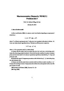
that the effect of 401(k) eligibility on financial wealth increases with age. The coefficient on e401k · (age − 41)2 is .060 (t statistic = 1.37), so it is not significant. The effect of e401k in part (iii) is the same for all ages, 14.219. For the regression in part (iv), the coefficient on e401k from part (iv) is about 8.357, which is the effect at the average age, age = 41. (d) . tab fsize, gen(fsize) family size | Freq. Percent Cum. ------------+----------------------------------1 | 203 21.88 21.88 2 | 217 23.38 45.26 3 | 198 21.34 66.59 4 | 188 20.26 86.85 5 | 74 7.97 94.83 6 | 31 3.34 98.17 7 | 11 1.19 99.35 8 | 5 0.54 99.89 13 | 1 0.11 100.00 ------------+----------------------------------Total | 928 100.00 . drop fsize5 fsize6 fsize7 fsize8 fsize9 . regress nettfa e401k inc incsq age agesq male fsize1 fsize2 fsize3 fsize4 Source | SS df MS -------------+-----------------------------Model | 1249291.04 10 124929.104 Residual | 3887629.61 917 4239.50884 -------------+-----------------------------Total | 5136920.65 927 5541.44622

Number of obs F( 10, 917) Prob > F R-squared Adj R-squared Root MSE

= = = = = =

928 29.47 0.0000 0.2432 0.2349 65.112

-----------------------------------------------------------------------------nettfa | Coef. Std. Err. t P>|t| [95% Conf. Interval] -------------+---------------------------------------------------------------e401k | 13.42462 4.595985 2.92 0.004 4.404754 22.44449 inc | -.5637908 .2564669 -2.20 0.028 -1.067121 -.0604606 incsq | .0142597 .001986 7.18 0.000 .0103621 .0181573 age | -1.732811 1.869153 -0.93 0.354 -5.401126 1.935504 agesq | .0321586 .0216034 1.49 0.137 -.0102393 .0745564 male | -1.783906 6.270077 -0.28 0.776 -14.08927 10.52146 fsize1 | 9.1958 8.194099 1.12 0.262 -6.885564 25.27716 fsize2 | 17.87712 7.54224 2.37 0.018 3.075066 32.67918 fsize3 | .5817076 7.547443 0.08 0.939 -14.23056 15.39397 fsize4 | 6.537835 7.612689 0.86 0.391 -8.402482 21.47815 _cons | 12.91241 39.44122 0.33 0.743 -64.49313 90.31795 -----------------------------------------------------------------------------. test fsize1 fsize2 fsize3 fsize4 ( ( ( (

1) 2) 3) 4)

fsize1 fsize2 fsize3 fsize4 F(

4,

= = = =

0 0 0 0 917) =

2.25

8

Prob > F =

0.0620

I chose f size5 as the base group. The estimated equation is da = nettf

12.912 + 13.425 e401k − .564 inc + .014 inc2 − 1.733 age + .032 age2 (39.44) (4.60) (.256) (.0020) (1.869) (.022) − 1.784 male + 9.196 f size1 + 17.877 f size2 + .582 f size3 + 6.538 f size4 (6.27) (8.19) (7.54) (7.55) (7.61)

n = 928, R2 = .243. The F statistic for joint significance of the four family size dummies is about 2.25. With 4 and 917 df , this gives p-value = .062, so they are not jointly significant. (e) Code not shown. The F statistic for the test of all 20 restrictions is 3.54, which with 20 and 9,245 d.f. has a p–value of essentially zero. Therefore, the constraints that all slopes are equal across family size groups are not warranted.

9