13th World Conference on Earthquake Engineering Vancouver, B.C., Canada August 1-6, 2004 Paper No. 1014

EARTHQUAKES GENERATION METHOD BASED ON FRACTAL GEOMETRY R. MAGAÑA1, A. HERMOSILLO2, M. ROMO3, G. SANTIAGO4 y M. PÉREZ5

SUMMARY In this article a procedure based on fractal methods is developed to generate synthetic signals. A revision is made of the procedures used to generate curves and fractal figures. Also a brief description of other methods to generate synthetic signals is presented. It should be emphasized that the fractal techniques are very appropriate to model natural phenomena (among them earthquakes). The proposed method allows, when varying some characteristics of the procedure, to generate synthetic signals having response spectra witch is compatible to design spectra proposed construction codes. This procedure is compared with results in terms of response spectra provided by synthetic signals (generated by other methods). Dynamic analysis will be made on simple structures of one, two and three degrees of freedom. INTRODUCTION A procedure based on fractal techniques to generate synthetic earthquakes is developed herein. This was accomplished with a large number of procedures to generate curves, and fractal figures of any kind were tried. For completeness other procedures to generate synthetic signals are also included. The proposed method allows a continuous change of some characteristics of the fractal procedure to generate synthetic signals having a specific target response spectrum. In chapter 2, some of the works found in Internet that deal with this problem are discussed. These included some articles where fractals used to generate music. From a mathematical point of view, these are similar in most aspects when applied to earthquakes. It is worth mentioning that fractal algorithms are also used to study vital signals in the human body. 1

Project Scientist, Institute of Engineering, UNAM, [email protected] Assistant research, Institute of Engineering, UNAM, [email protected] 3 Head, Geotechnical Department, Institute of Engineering, UNAM, [email protected] 4 Assistant research, Institute of Engineering, UNAM, [email protected] 5 Professor of ENEP Aragón, UNAM, [email protected] 2

In chapter 3 the technique to generate signals from different fractal figures are shown. In chapter 4 a fractal algorithm to generate synthetic signals developed with Matlab, is shown. Chapter 5 includes an algorithm developed by the authors at the Institute of Engineering. In Chapter 6 it is presented a method for the analysis of signals with the method of phase space diagrams. In chapter 7 is presented some final comments. SIGNALS FRACTAL GENERATION Basic concepts In the book "Fractal geometry of nature", by Benoit Mandelbrot (ref 1), the fractal concept was employed to affirm that, the Euclidian geometry is not useful to represent many aspects of nature. Two characteristics have to be fulfilled by a fractal: self-similarity and fractal dimension (besides there is not a unique derivate in any point of a fractal curve). In his book, Mandelbrot sustains that there are two kinds of fractals: the linear and the complex. The linear fractals are built from linear algorithms (e.g., Sierpinsky’s triangle) and the complex making iterations with formulas within the field of complex functions (e.g., Mandelbrot and Julia's sets (ref. 1)). The dimension of self-similar objects (called Hausdorf-Besicovitch) is a generalization of the Euclidean one and is represented by the following formula: S=LD, where S is the segment’s longitude, L is the measure scale and D is the dimension. Another important parameter in fractal geometry is the Hurst’s exponent (ref 2), which is linked with the fractal dimension by means the expression: H = 2-Fd Another useful variable to measure the diversity of values that acquires a fractal curve is called entropy. It is represented by the Shannon-Weaver’s expression (ref 3): E = − pi ln pi

∑ i

Where pi is the probability that an experiment had the “i” value, p i = ni / N , where N is the total number of experiments and ni is the number of times that a particular experiment had the value or class i. The minimum value of “E” appears when all the elements have the same value, in this case E=0. Classification criterion This criterion consists on calculating for each real or synthetic signal two parameters, its fractal dimension and its entropy (this concept was commented in chapter 2), each signal is located as a point within a system of reference, the entropy value is represented in the abscissas and the fractal dimension in the ordinates. How to get the fractal dimension of seismic signals To get a synthetic signal using the method of the spectral synthesis based on Fourier's transform, it is necessary to calculate the Hurst's coefficient (H). This coefficient should not be arbitrary; it is calculated using the relation that it exists between the fractal dimension Fd and the H coefficient of same time series. This relation is H = 2 – Fd. To obtain the Fd of the some time series, and after obtaining the H coefficient. In table 1, where the Fd is calculated for 5 time series, three real and two synthetic signals generated witch the Gasparini y Vanmarcke’s method (ref 4).

Earthquake

Duration (seg)

Fd

CSER9906151E O LZ089412101EO

134.41

1.485

66.55

MZ079510092EO

15.45

synthetic 1

129.45

synthetic 2

112

1.364 1 1.346 4 1.516 8 1.513 7

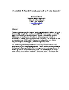
Table 1 Fractal dimensions of earthquakes used in this analysis It is necessary to clarify that the box-counting method is used for time series that are self-similar. The time series presented here are self-similar. If we plot the fractal dimension and the entropy for each one of the analyzed time series (fig 1) we can see more disorder or entropy present in a seismic signal, as the accelerations set associated to the signal is more erratic.

Figure 1 Fractal dimension and entropy of the analyzed seismic signals Generation methods In the document “Discovering fractals” (Francisca Muñoz y Rodrigo Meza) (ref 5), it was found a link between music and fractals, which is expressed in the following paragraph. The work, “Real time transformation of music with fractal algorithms” (ref 6), is an account of four musical fragments during the period 1988-1993: “The fractal mountains” (1988-89), “The summer song” (1991), “The mountany song” (1992) and Goss (1993). Gordon Monro in his work (ref 7), “SOME EXPERIENCES WITH ALGORITHMS IN MUSIC COMPOSITION” presents his experience using algorithms with musical composition and comments that the algorithms can be divided into two main types: a) Algorithms that determine the notes yielding the musical fragment, and b) Algorithms that produce the actual forms of the sounds that we hear commonly. Kits for fractal creations The following Internet references are a good place to be introduced in this topic:

1) Interesting links about the Fractint program. The Fractint welcome page: http://spanky.triumf.ca/www/fractint/fractint.html and the Fractint’s tutorial: http://areafractal.tierradenomadas.com/fctint.html 2) Ultrafractal, to download the program, we can get it from: http://www.ultrafractal.com Of course Fractint and UltraFractal are only two of the hundreds of programs to generate fractals. Some others that are convenient to point out are: -Fractal Explorer, Can be downloaded from: http://www.eclectasy.com/Fractal-Explorer/index.html -Fractal Music by Michael Lloyd (ref 8). In this article he discusses a mathematical definition of a pair of fractals. SIGNALS GENERATION FROM FRACTAL FIGURES

From the concepts used for the music generation by means of fractals images we can create signals starting from fractal images. It is known that a fractal is the iteration of a simple algebraic expression (ref 9). The image usually seen with colors and forms is the representation of this iteration within a graphic environment within a complex plane, by means of special programs. Each image is composed by a enormously high number of points which plotted in the plane form each fractal. If we associate a music note to each point, we will obtain fractal music. Geometrically, a fractal is generated by a pattern or generator (ref 9). An example of music generation using Mandelbrot’s set is the following: (1) Numbers are mapped to simple tones (ref 10); (2) The numbers are obtained from the Mandelbrot portion in the following image:

Figure 2 Mandelbrot fractal

Figure 3 Generated signal

The sound files are simple illustrations of audible data. We can imagine a microphone moving along a line of the image. Each image pixel has a number value. As we scan a pixels line, the numerical value of each pixel is mapped sequentially to a set of tones. The values that determine the played tones and its duration should be specified. When scanning a line on the fractal image, we obtain the figure 3.

Fractalization One of the methods most used to generate of fractal music is through the repetition of an initial pattern of notes (ref 11). Starting from each one of them a new set of notes can be generated, following the same initial pattern, but giving more velocity and time variation. Hence, from this, identical repetitions from the original pattern other notes are obtained, but in another time and tone scale. There are two ways to generate signals from fractal figures: 1) Starting from fractal images, 2) Following an iterative process that generates the fractal. The former, simply scans on the fractal image following lines or curves in an arbitrary way. The corresponding color number to each scanned point is written in a file; the color intensity will represent a peak in the generated signal. The second procedure consists on generating the signal at the same time the fractal is being built. During the iterative process, we can

indicate to the program that stores in a file the number of iterations corresponding to each point belonging to the scanned line or curve. Signals obtained from fractal images using line segments are shown in the following images. Mandelbrot’s Fractal This fractal is built iterating the expression Z = Z2 + C, where Z is a complex variable and C is constant. The signal was made writing in a file the iterations corresponding to each one of the points corresponding to a straight line segment. Mandelbrot's signal

Iteration

300 200 100 0 -100 0

50 Pixel

100

Figure 4 Sector of a Mandelbrot’s fractal (left) and a generated signal through a line (right).

Newton’s Fractal This fractal is built iterating the equation p(z)-1=0 (ref 12). The generated signal was obtained writing in a file the corresponding iterations to each one of the points belonging to a straight line segment.

Iteration

80 60 40 20 0 0

200

400

600 Pixel

800

1000

Figure 5 Newton’s fractal and his generated signal

The Lorenz Attractor This attractor is built varying and iterating the following equation system:

∂x ∂y ∂z = ∂( y − x ) , = rx − y − xz , = xy − bzz ∂t ∂t ∂t To generate a signal with this fractal, the image is built and over it we scan a line. In the following image the generated signal is shown:

80

Iteration

60 40 20 0 -20

0

200

400

600

Pixel

Figure 6 Lorenz Attractor and the generated signal from a straight line segment that crosses the atractor Results obtained from fractal figures Next some generated signals using the Mandelbrot’s fractal will be shown; on a specific zone we scan throughout a line segment three different times. For each signal its response spectrum is calculated. Also the fractal dimension and entropy of the generated signals are shown with their respective response spectra.

Spectrum 1 200

150

150

a (m/sec²)

a (m/sec²)

Signal 1 200

100 50 0

100 50 0

0

20

40 t ime, sec

60

80

Figure 7 First scanning, a little magnification Fractal dimension: 1.00, Entropy: 2.76 Signal 3

150 100 50 0 100 time, sec 200

0.5

300

Figure 9 Third scanning, bigger magnification Fractal dimension: 1.21, Entropy: 2.83

1

1.5 time, sec

2

2.5

3

Figure 8 Response spectrum of the first signal Fractal dimension: 0.97, Entropy: 1.76 Spectrum 3

300 250 200 150 100 50 0

200

0

0

0

1

2

3

time, sec

Figure 10 Response spectrum of the third signal Fractal dimension: 1.01, Entropy: 2.29

Newton´s fractal Related to Newton’s fractal, we scanned a straight line segment. Each time we zoomed the image, three signals were obtained. Only the signal and spectrum corresponding to the third scanning is shown below.

70

100 a (m/sec²)

60 50 40 30 20 10

80 60 40 20 0

0 0

100

200

300 time, sec

400

0

500

Figure 11 Third scanning, bigger magnification Fractal dimension: 1.25, Entropy: 1.80

1

2 time, sec

3

Figure 12 Response spectrum of the third signal Fractal dimension: 0.96, Entropy: 1.84

We can distinguish certain tendencies for from which fractals. The tendencies are proper of each fractal, and the response spectra, corresponding to each one, are different among them. SIMULATION OF SIGNALS WITH A FRACTIONAL BROWNIAN MOVEMENT In this chapter a method to generate a fractional Brownian movement (fBm) is presented. This method is named spectral synthesis based on the Fourier’s transform. The generated fBm is modulated by an envolving curve, then the generated signals present characteristics of fractal dimension and entropy very similar to these actual seismic signals. In 1968 the concept of fractional Brownian movement (fBm) (ref 13) was introduced as a movement which is a random function X(t), the increments of which in a time interval, have a gaussian distribution, when the mean squared increases or variance satisfies the equation:

E (( X (t ) − X (t 0 )) 2 ) = k t − t 0

2H

Then the fBm is a non stationary stochastic gaussian process with mean = 0, whose main statistical properties depend on the time. The H index is a parameter know as the Hurst’s exponent that varies from zero to one. When this exponent has a value of 0.5, a Brownian movement is obtained. For H values larger then ½, the tendency of the time series either has an upward or downward development. This behavior is more notorious when H approaches to one. A lower exponent than ½ indicates no-persistence (erratic behavior). Generation procedure Different methods have been used to generate a fBm. They can be classified in two categories: middle point displacement methods and synthesis spectral methods. Both methods uses generators of random numbers, so that a correlation level (fixed when selecting “H”) is maintained. Now we are going to describe the synthesis spectral method to generate a fBm: Given a periodic function X(t) where t varies between 0 and 2π, provided that X(0) = X(2π), it can be written:

X (t ) =

∞

∑C e π

2 int

n

n = −∞

where Cn are independent Gaussian random coefficients. These coefficients should fulfill the following conditions:

a) |Cn| values are independent and are normally distributed with zero mean and variance equal to

E Cn

2

=

1 2 E ( C1 ) , 2 n

n>0

b) The arg(Cn) variables (phase angles) are independent and uniformly distributed in (0, 2π). For a generalized Brownian motion with Hurst’s exponent H, the variance is 2

2

E ( C n ) = E ( C1 )n −1− 2 H ,

n>0

So that the power spectra satisfy an exponential law to the power of (-1-2H) To perform the synthesis of fBm, the following steps should to be performed: 1. The H exponent value is selected, which must be 0 < H < 1. 2. The quantity of N terms that are going to be used in the simulation is established (Fourier's coefficient). Notice that N is the highest frequency implied. Choose N phases in ϕ1, …, ϕN, randomly distributed [0,2 π] 3. The |Cn| amplitudes are selected from normally distributed samples with zero mean and variance proportional to n-1-2H. 4. The spectrum |Cn|exp(iϕn) is established. 5. The Fourier inverse transform (ifft) is applied to obtain a complex fractal process. The number of points in the resultant signal follows when the method is applied.

The obtained signal in the last step presents a form that is congruent with the elected Hurst's exponent. To modulate the fBm form an enveloping function is applied, which is calculated starting from the energy of seismic signals. One of these signals is shown in the figure 13.

Figure 13 Fractional Brownian movement with H = 0.61 with wrapping One of the parameter that can be modified so that the resultant signal has different characteristics, is the definition of the maximum frequency of the Fourier's spectrum, which can be calculate as: f max = N = 1/(2∆t ) where we can see that this frequency depends on the digitalization interval, ∆t, of the signal. The frequency parameter is related to the duration of the resultant signal, which can be also modified to obtain signals of various durations. These three parameters (Maximum frequency, digitalization interval and signal duration) should be modified at the same time to obtain signals with different characteristics.

Another parameter that could be varied angle phases, this can be accomplished analyzing Phase Fourier Spectra of different signals. Examples of generated signals We are going to explain the procedure to generate signals that can be considered as the fractional Brownian movement. These signals are modified so that they show some of the characteristics from the real seismic ones. Once that the fBm’s were calculated their ordinate values were multiplied to get similar acceleration values to those of seismic records. The scaling factor was 10.00. In this case a maximum value of 200 cm/seg2 in the fBm was selected. Figure 14a represents an fBm generated with a value of H = 0.61392. For the sake of comparison, the original motion is included on the left side of the figure.

Figure 14 Fractional Brownian movements generated with H = 0.61392

The entropy and fractal dimensions of the time series shown in figure 14, were computed to assess their pertinence of actual seismic events. The Fd and the entropy of fBm of the signals (also included in table 1) are shown in figure 15.

a) Actual events

b) Synthetic signals

Figure 15 Fractal dimension and entropy of fractional Brownian movements

PROPOSED FRACTAL ALGORITHM Background To elaborate the algorithm different ideas from the fractal geometry theory and works of different authors were taken into account; for this reason, some of then are discussed first. One of the basic ideas of the fractal geometry is the use of iterative algorithms with the basic geometrical components, like the initiator and generator elements. In (ref 14) these principles are used. They present a fractal graph named Devil’s staircase witch is generated by an iterative application of the next equations:  1  1 f (3x) si x ∈ 0,   2  3   1 1 2  Tf ( x ) =  si x ∈  ,  2 3 3   2  1 1  2 + 2 f (3x − 2) si x ∈  3 ,1 

With these expressions graphs such as those shown below are obtained.

Figure 16 The devil's Note that the figure on the right has roughly the configuration of a time history (i. e., accelerogram).

1

0.6

0.5

0.4 0.2

0 0

10

20

-0.5

0 -0.2 0

1

10 20 time, sec

Figure 17

30

30

a (m/sec²)

0.8 a (m/sec²)

a (m/sec²)

Procedure To develop the algorithm, a segment of a horizontal straight line is used as starting element and as generator different patterns can be used. In figures 17 to 19 some simple patterns are shown.

0.5 0 0

-1

5

10

15

20

-0.5 time, sec

Figure 18

time, sec

Figure 19

It is possible to use a great variety of patterns. Furthermore, it is possible to use some patterns scanned from actual earthquakes. This is part of an ongoing research. As an example, in figures 20 and 21, the first three iterations, using the simple pattern of figure 17.

1

1.5

a (m/sec²)

a (m/sec²)

1

0.5

0 0

5

10

15

20

25

30

0.5 0 -0.5 0

10

20

30

-1

-0.5

-1.5 time, sec

time, sec

Figure 21

Figure 20

Variants The proposed method allows signal generation using different control elements: a) Pattern used, b) Quantity of subdivisions, c) Quantity of iterations, d) Time discretization, e) Scale factor, f) Generated forms from earthquakes patterns.

Results from the developed algorithm. By means of the program developed for the generation of fractal signals, we obtained several signals varying the number of divisions and the number of iterations. From each signal its fractal dimension and entropy was obtained are shown in figures 22 to 24.

1

1.5

0.5

0.5

a (m/sec²)

a (m/sec²)

1

0

0

50

100

-0.5 -1

0 -0.5 0

20

40

60

80

100

-1 -1.5

time, sec

time, sec

Figure 22 Signal 1, 5 divisions, 2 iterations Fractal dimension: 1.076, Entropy: 3.41

Figure 23 Signal 3, 7 divisions, 2 iterations Fractal dimension: 1.30, Entropy: 3.65

1.5

a (m/sec²)

1 0.5 0 -0.5 0

20

40

60

80

100

-1 -1.5 time, sec

Figure 24 Signal 4, 21 divisions, 1 iteration Fractal dimension: 1.53, Entropy: 4.29

Of the previous graphs it can be concluded that modifying the number of divisions or iterations we can alter the fractal dimension and the entropy. It should be mentioned that synthetic time series can be developed using other advanced techniques such as fast diagrams (ref 15) ANALYSIS OF SIGNALS WITH THE METHOD OF PHASE SPACE DIAGRAMS The phase space diagrams are tools that help to interpret the topology and the evolution of the solution. It is possible to construct it with the original series and with delays in the time of the same one. a sequence of experimental observations in its simpler form, produces a time series: a list of numbers that represent the value of the magnitude observed in regular intervals of time. For example, the daily temperature in a given place at noon forms a time series, perhaps one like this: 17.3, 19.2, 16.7, 12.4, 18.3, 15.6, 11.1, 12.5..., in degrees Celsius. If we want to fit these data to a strange attractor, we have the problem to have data of a single magnitude whereas we required three. What Ruelle and Packard understood was that two additional observable fictitious can be obtained from a single time series, moving the value of the time. Instead of the unique time series three are compared; original and the two copies, moved one and two intervals, respectively: Series 1

17.3, 19.2, 16.7, 12.4, 18.3, 15.6, 11.1, 12.5,…

Series 2

19.2, 16.7, 12.4, 18.3, 15.6, 11.1, 12.5,…

Series 1

16.7, 12.4, 18.3, 15.6, 11.1, 12.5,…

According to the time evolves, these tuples move in the space. Ruelle y Packard conjectured that the ways that draw up these tuples are a topological approach to the form of the attractor. The attractors can be classified in constant, periodic, quasiperiodic, chaotic and random, as they are show in the following image (figure 25):

Figure 25 Attractors classification The constant attractors only contain a point, which indicates that all the values are equal, the periodic ones generate a figure simple as a circumference, the quasiperiodics ones move in the neighborhoods of periodic attractors.

In the time series of random data, patterns are not observed, nor particular geometries. The chaotic data generate strange attractors. We applied this technique to different seismic data, with the following results (figure 26):

Figure 26 Real accelerogram. A very ordered distribution is observed, susceptible to found patterns

FINAL COMMENTS a) Investigation and applications of fractal geometry carried out, up to now to generate synthetic signals of any type is very extensive (among them of earthquakes). b) The procedure to generate signals starting from fractal figures is very versatile, because many signals of different types can be generated, since the gallery of fractals figures is very ample. c) In MATLAB yields a great possibility to generate fractal synthetic signals and also using mathematically based methods. d) The algorithm developed is very simple and it is versatile enough to be adapted to generate signals with characteristics very similar to actual earthquakes. e) As observed in the diagram of phase states, actual earthquakes show some chaotic characteristics and can therefore be modeled with fractals. f) The proposed criterion, based on the reference system (fractal dimension versus entropy), is objective and it allows making comparisons between real and synthetic signals.

REFERENCES 1. 2. 3. 4.

5. 6. 7.

Mandelbroot B. B., “The Fractal Geometry of nature”, Freeman: San Francisco 1978. Internet direction: http://www.etsimo.uniovi.es/ Felicísimo, Angel Manuel, internet direction: http://www.etsimo.uniovi.es/ Gasparini D. and Vanmarcke, “Simulated earthquake motions compatible with prescribed response spectra”, Massachussets Institute of Technology.. Department Civil of Engiineering. Report Non R76-4, 1976 Muñoz F. and Meza R. “Descubriendo los fractales”, internet direction: http://www.dcc.uchile “Real Time Transformation of Musical Material Fractal with Algorithms”. internet direction: http://www.timora.con.charlin.edu/ Monro G. internet direction: http://www.gordonmonro.com/misc/acoustic-ecology.html

8. 9. 10.

11. 12. 13. 14.

15.

Lloyd M. “Fractal Music”, internet direction: http://www.hsu.edu/faculty/afol200203/contents2D.htm-19k Muñoz F. and Meza R. “Discovering the fractals”, I Project computer graph - cc52B Formless Number 1, Sciences Dpt. of the Computation FCFM-OR. of Chile. Muñoz F. and Meza R. The fractal one, the random cloud, the algorithm of the half point and their music. Computer project Graph-CC52B. Formless Number 3, Sciences Dpt. of the Computation FCFM-OR. of Chile. “Fractal music”, internet direction http://www.oni.escuelas.edu.ar/2002/buenos_aires/infinito/arte.htm Stevens, Roger T. “Fractal Programming and Ray Tracing With C++”. M & T Books, States United of America, 1991 Mandelbroot B. and Van Ness J. “Fractional Brownian motions, fractional Gaussian noises and applications”, SIAM rev. Appl. Math., Vol 10 Not 4 pp427-437, 1968 Ferreol R. and Mandonnet J. “Escalier du diable.” Internet direction: http://www.mathcurve.com/fractals/escalierdudiable/escalierdudiable.shtml-9k, 2002 Translation, Ortuño M., Ruiz Martínez J. et al, ¿Juega Dios a los dados? The new mathematics of the Chaos. Grijalbo Mondadori S. A. ed, Barcelona. 1991