Abstract This project is a 30 ECTS master thesis for Kjetil Fløisand S041939 and Kristian Lund S041947 in the period of the 24th of February to the 31st of July, 2006. It is done in cooperation with ABB and DTU (Technical University of Denmark). The project is performed under guidance of Morten Lind from DTU and Lars Knudsen from ABB. This report is about implementing a commercial product for ABB. In order to not make this product’s information available for rival firms of ABB, it has to be kept classified. Frederiksberg fjernvarme is a district heating supplier for Frederiksberg in Copenhagen, which uses ABB’s system to monitor and control their pipes, pumps, valves and other components involved in their network concerning the district heating system. Their current monitor system has a geographical relation with the components actual location in the field, thus they have some new specifications for a more advanced and lucid geographical system. On behalf of the new system requirements, ABB is developing a new district heating network monitoring system, with an integrated Hydraulic Calculation Model (HCM). A HCM is a system, developed by an external vendor (-not ABB), which is commonly used to dimension components in a district heating system. In a HCM it is possible to build up a model of a district heating system and then simulate the behavior of the system (temperature, pressure, flow etc) on behalf of the pipe dimensions, valve states, consumers, producers etc. In this project its purpose is to calculate behavior and states of the system, which are not available from sensors. The new system that is to be delivered will be build around ABB’s platform 800xA, and have the ability to supervice the district heating network on a detailed plan, as well as simulate changes in the system. Our master thesis is about building up a service application for a HCM delivered by 7-Technologies, with an OPC interface. On the base of this, our main issue is divided into two. 1. Build the OPC server to communicate with the 800xA platform. 2. Build a COM interface to communicate with the HCM from 7-Technologies. This report describes how the project is analyzed and designed. The report is consisting of three main parts. The first part of this report gives an introduction to the problem. The second part is about the requirements and design of the HCM application. The third part is about the implementation of the application. We started cooperation with ABB concerning our master thesis on the purpose of testing our skills in a commercial company. Hopefully, this project will serve a purpose for ABB. We will therefore give a huge thanks to Lars Knudsen and Torben Andersen at ABB for their patience and helpfulness giving us, and helping us through, this project.

1

Dynamic Network Modeling Abstract ................................................................................................................................................1 1 Introduction.......................................................................................................................................5 1.1 Background ................................................................................................................................5 1.2 New system demands.................................................................................................................5 1.2.1 Detailed dynamic system information ................................................................................5 1.2.2 Simulation ...........................................................................................................................6 1.2.3 Zooming and Panning .........................................................................................................7 1.3 Problem formulation ..................................................................................................................7 1.3.1. The hydraulic calculations models COM interface............................................................9 1.3.2. The hydraulic calculations models OPC-Server ................................................................9 1.3.3 The HCM’s service application ..........................................................................................9 Performance specification......................................................................................................10 1.4 Demarcation .............................................................................................................................10 1.5 Method .....................................................................................................................................10 2 District heating network..................................................................................................................12 2.1 Physical network ......................................................................................................................12 3 Technical solution ...........................................................................................................................14 3.1 Super ordinate system description ...........................................................................................14 3.2.1 Server system ....................................................................................................................14 3.3.2 Dataflow............................................................................................................................16 4 Project technologies ........................................................................................................................18 4.1 COM interfaces and objects.....................................................................................................18 4.2 Termis Hydraulic Calculation Model from 7-Technologies....................................................19 4.2.1 Modeling the network .......................................................................................................19 4.2.2 Communicating with the Termis model............................................................................20 4.2.3 Operating the Termis model in Outtake............................................................................20 4.2.4 Component description .....................................................................................................22 4.3 OPC (OLE for Process Control) server....................................................................................24 4.4 Northern Dynamic Inc toolkit v3.0 ..........................................................................................26 4.5 ABB’s industrial IT system, 800xA.........................................................................................28 4.6 DNM Configuration database ..................................................................................................29 5 Design of the OPC tree structure ....................................................................................................31 5.1 The OPC tree structure.............................................................................................................31 5.2 OPC item types ........................................................................................................................32 5.2.1 Value Item.........................................................................................................................32 5.2.2 Boundary Item...................................................................................................................33 5.2.3 SetReset Item ....................................................................................................................33 5.2.4 Update Item.......................................................................................................................33 5.2.5 ResetAll Item ....................................................................................................................33 5.2.6 StartSimulation Item .........................................................................................................33 6 Designspecifications for implementation of HCM .........................................................................34 6.1 Running....................................................................................................................................35 6.1.1 Online................................................................................................................................35 6.1.1.1 Reading boundary conditions from 800xA................................................................36

2

6.1.1.2 Updating HCM...........................................................................................................37 6.1.1.3 Boundary classes........................................................................................................38 6.1.1.4 Updating Thread ........................................................................................................39 6.1.1.5 Update the OPC items................................................................................................40 6.1.2 Simulation .........................................................................................................................41 6.1.2.1 Change the OPC items to writeable ...........................................................................43 6.1.2.2 Save the changed boundary conditions......................................................................44 6.1.2.3 Update HCM with boundary conditions from 800xA ...............................................45 6.1.2.4 Update HCM with simulated boundary conditions....................................................45 6.1.2.5 Calculating the simulation .........................................................................................46 6.1.2.6 Reset all boundary conditions ....................................................................................46 6.2 Startup ......................................................................................................................................46 6.2.1 Reading the Configuration database .................................................................................47 6.2.2 Building the HCM models ................................................................................................48 6.2.3 Building the Boundary objects..........................................................................................49 6.2.4 Building the OPC tree .......................................................................................................49 6.2.5 Building the ControllSimulation objects...........................................................................51 7 Implementation ...............................................................................................................................52 7.1 Startup ......................................................................................................................................52 7.1.1 Reading the configuration database ..................................................................................54 7.1.2 Building the boundary objects ..........................................................................................57 7.1.3 Reading boundary conditions from 800xA.......................................................................60 7.1.4 Building HCM...................................................................................................................63 7.1.5 Build the OPC tree ............................................................................................................67 7.2 Running....................................................................................................................................70 7.2.1 Online................................................................................................................................70 7.2.1.1 Update the HCM ........................................................................................................70 7.2.1.2 Update the OPC items................................................................................................73 7.2.2 Simulation .........................................................................................................................76 7.2.2.1 Controlling the Simulation.........................................................................................76 7.2.2.2 Toggle access right.....................................................................................................79 7.2.2.3 Save the changed boundary conditions......................................................................80 7.2.2.4 Calculate a simulation................................................................................................82 7.2.2.5 Reset all......................................................................................................................84 7.2.2.6 Update the simulation model .....................................................................................85 8 Testing and debugging ....................................................................................................................87 8.1 Test on Online calculations......................................................................................................87 Test scenario I ............................................................................................................................89 Test scenario II...........................................................................................................................90 Test scenario III .........................................................................................................................91 Test scenario IV .........................................................................................................................93 Test scenario V...........................................................................................................................95 8.2 Test Simulation ........................................................................................................................96 Test scenario VI .........................................................................................................................96 Test scenario VII........................................................................................................................98 Test scenario VIII.......................................................................................................................99 Test scenario IX .......................................................................................................................101

3

8.3 Non compliant OPC server ....................................................................................................106 8.4 Memory leak and garbage control .........................................................................................106 9 Conclusion ....................................................................................................................................108 10 Perspective ..................................................................................................................................109 Appendix A ......................................................................................................................................110 1 Class definition .........................................................................................................................110 HydrMod..................................................................................................................................110 Operation Specification........................................................................................................110 BoundaryReadClass .................................................................................................................125 Operation Specification........................................................................................................125 BoundaryConditionThread.......................................................................................................127 Operation Specification........................................................................................................127 DNMConfHandler ...................................................................................................................133 Operation Specification........................................................................................................133 Boundary class: ConsumerBound ............................................................................................139 Operation Specification........................................................................................................140 Boundary class: HeatExchangerBound....................................................................................142 Boundary class: HeaterBound..................................................................................................143 Boundary class: NodeBound....................................................................................................144 Boundary class: ProducerBound ..............................................................................................145 Boundary class: PumpBound ...................................................................................................147 Boundary class: ShuntBound ...................................................................................................148 Boundary class: ValveBound...................................................................................................149 BuildOPC .................................................................................................................................150 Operation Specification........................................................................................................151 HNODE_Cl..............................................................................................................................158 Operation Specification........................................................................................................158 Controlsimulation.....................................................................................................................167 Operation Specification........................................................................................................168 SimulationData.........................................................................................................................171 Operation Specification........................................................................................................172 HCMServerCallback ................................................................................................................181 Operation Specification........................................................................................................182 2 Schedule ....................................................................................................................................185 Appendix B, On CD.........................................................................................................................186 1 HCMOPCServer, the program..................................................................................................186 2 ABB’s project description.........................................................................................................186 3 7-Technologies’ Termis’ COM interface..................................................................................186 4 Outtake ......................................................................................................................................186 5 Flowcharts for outtake ..............................................................................................................186 6 Northern Dynamic Toolkit V.3.0..............................................................................................186 7 Test scenarios............................................................................................................................186

4

1 Introduction 1.1 Background For district heating suppliers it is crucial that the heated water distributed to their clients are within a specific temperature range. The same goes for pressure and flow, but only temperature is described in this section. To keep the water temperature in the specific range, several automated control systems are used. These control systems works well in most cases, but can fail as any other technical equipment. In a situation of failure it is important for the district heating suppliers to get this knowledge as fast as possible. Further on, the district heating suppliers wants to know the exact geographical locations where the temperature has dropt as a cause of a failure. This information gives them the possibility to notify the actual clients about the problem, and take action to prevent further problems. An improved general view of the network gives an enhanced process. For Frederiksberg fjernvarme there is made a geographically monitoring system based on maps of the area where the district heating network is located. In these maps, dynamic symbols that show the state of water pipes, valves, pumps and sensors are placed according to their location. The symbols change their color after the actual state. For instance, the pipe symbols are red when the water is warm and blue when the water is cold. With these maps, an operator can view the states of the district heating network according the geographical location. The existing geographically monitoring system is called DNM. For all modern district heating networks there is made a Hydraulic calculation model. The Hydraulic calculation model (HCM) is a mathematical model of the physical network. Originally the HCM was intended for aid when constructing the networks, but can to day be used for simulation and system-state calculations. ABB wants to develop a monitor system for district heating network which integrates a HCM.

1.2 New system demands This report describes a subtopic of the larger project that is to be developed by ABB. Therefore to get a better understanding; the next section gives a short description of the goals of the entire project. ABB are going to develop a new geographically monitoring system in cooperation with Frederiksberg fjernvarme called DNM2. DNM2 shall be one of ABB’s products, based on ABB’s 800xA platform and have SCADA functions (alarms, historic, trend, and e.g.). DNM2 shall have three new properties: dynamic system information, simulation and zooming and panning.

1.2.1 Detailed dynamic system information The dynamic information of the network states that are displayed on the maps will be more detailed. There are a huge number of sensors in the system measuring the network states. But compare to the physical size of the network, there are very few sensors. The temperature in middle of two sensors

5

can only be assumed at best. If the temperature for one of the sensors decline, what happen with the temperature in the middle? This uncertainty gives a problem with the desire to be able to know which clients that are affected by a temperature drop. To be able to solve this problem, the HCM for the district heating network that already is developed is used to calculate more state variables. The HCM’s calculated variables give a more detailed picture of district heating network.

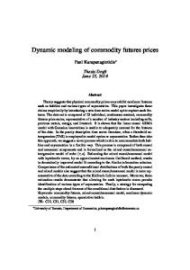
1.2.2 Simulation There will be made a simulation mode for the geographical monitoring system, where different scenarios can be tested. That is, an operator shall be able to test the result of changing different system states. For example, what happens if a valve is closed or a pump is stopped? The advantage of knowing the effect of such an action before it is made cannot be overestimated. Different ways to solve the same task can be simulated, to find the best solution. The simulation shall also show which clients that will be affected by a change of a system state. This could be used to notify the actual clients before they are affected. The HCM that calculates the virtual states shall also be used for simulation. In simulation mode the HCM will takes measured values as boundary conditions except for the values that are to be simulated (valve position, pump speed, e.g.) to calculate simulated values. The simulation mode shall be made such that several users can simulate different scenarios at the same time. The number of simultaneous performable simulations shall be decided by a configuration database.

6

Figure 1.1 illustrates four users connected to DNM2.

1.2.3 Zooming and Panning The maps shall be made more flexible with the possibility of zooming and panning. The existing maps have no possibility for zooming, something that is very advantageous in a larger city. With zooming, information can be hidden in one level and then displayed when zoomed in. This gives a more lucid display. The information can be very detailed in the closest zoom mode, such as street names, contact addresses and phone numbers as well as names of pipes, pumps, valves etc. To be able to perform the zoom effect in to a map, one needs numerous maps, one for each zoom level. Al these maps must be arranged in a database. The correct map must be selected for each level. For each map the right information must be assigned, such as dynamic symbols, street names and so on. The dynamic symbols used in the maps shall have the same properties as SCADA symbols, such as alarms, trend, history, link to technical specifications and so on. Both the real and the virtual states shall be shown with dynamic symbols, and the user must be able to see the difference between these types of states.

1.3 Problem formulation This project consists of a subtopic of the project that ABB is developing, which is concerning the integration of the hydraulic calculation model (HCM) into the 800xA system. To include the HCM

7

in the 800xA system, a service application is needed. The service application is to be implemented by the C++ programming language, using COM and OPC interfaces. This service application has two main parts; online calculations of virtual states based on real-time process values, and giving users the possibility of simulating changes in the district heating network. Online The service application will read boundary conditions (real-time process values) from 800xA, and sends them to the HCM for calculations. The service application shall then make the calculated values available for 800xA with an OPC interface. Simulation The service application will read boundary conditions from both 800xA and the simulated values from an OPC interface, and sends them to the physical HCM for calculations. The service application shall then make the calculated values available for 800xA with an OPC interface. Startup Besides this, the service application has to receive configurations from a configuration database at start-up. This configuration holds the physical description of the system, which values are boundary conditions, what kind of physical object etc.

Figure 1.2, a rough illustration of the service application The service application will be designed for reuse. That is, the DNM2 system is to be used for other district heating system with other HCM, thus it is also important that the COM interface is designed with the possibility to adapt to other HCM interfaces with a minimum of change. The service application shall be designed such that several users shall have the possibility to connect to the service application and perform different simulations. The number of possible

8

simultaneous simulations is defined in the configuration database. The service application must adapt to the number of simulations. The service application are to be implemented as an application for the 800xA system, thus it needs an 800xA shell. The implementation of the service applications can be, in its preface, derived into two main parts, the HCM’s COM interface and the OPC server, which are two separated tasks. These two parts will later on be integrated in the same system, the service application for the HCM.

1.3.1. The hydraulic calculations models COM interface The HCM is delivered by extern producers and is not developed for communicating with ABB’s standard systems. A HCM is in fact a separately running program, a kind of server program. The extern producer in this case 7-Technologies uses the COM technology for communicating with the HCM (COM is developed by Microsoft to enable interprocess communication and dynamic object creation). The service application will therefor need a COM interface to communicate with the HCM. When the serviceapplication receives the physically structure of the system from the configuration database, it has to build up an analouge configuration in the HCM program. At run-time it has to send data for calculation to the HCM, and then receive the calculated values. The COM interface will be designed after the interface of the 7-Technologies HCM, and are to be implemented as an own class in the service application.

1.3.2. The hydraulic calculations models OPC-Server The 800xA system is tailored to communicate with OPC (OLE for Process Control) servers. Therefore it is essential that the district heating system states (measurements and estimates) are available as OPC items. OPC is based on the Microsoft technology OLE (Object Linking and Embedding) to make links between Windows based software applications and process control hardware. An OPC server will be designed to make the calculated values from the HCM available for the 800xA system. The 800xA system can then link these values to scada object etc. The OPC server will also be used to control simulations of the district heating network.

1.3.3 The HCM’s service application When the two parts are developed, they will be integrated into the service application. The service application will stand for the main logic of the calculation system. It will, at start-up create the OPC server and the hydraulic model, based on the data received from the configuration database. Thus, an interface to the database will be essential in this application. The OPC server will be build up with an online branch, which will have tags related to all of the virtual and measured values in the hydraulic model. The service application will, with a specific interval, receive the boundary values from the PLC’s via the 800xA system, and then feed the hydraulic calculation model with these values. The interface and the item tagging to the real PLC values must therefore have to be described in the configuration database to allow adoption to other district heating systems. After a calculation, the online branch will be updated with both the calculated, and the boundary values.

9

Beside the online branch, the OPC server will hold a number of simulation branches. The number of simulation branches will be specified by the configuration database, and is determining the number of simultaneously performable simulations. Each simulation branch will be identical to the online branch, but they will not be updated by calculations with the boundary values. When performing a simulation, the service application will feed the hydraulic calculation model with boundary conditions received at the simulation branch of the OPC server, and not from the PLC values like the online calculation. The simulation branch will then be uploaded with the calculated values in the same way as the online branch, but it will contain values related to the simulation and not the real states of the district heating system. This means, each simulation branch will both hold the input to, and output from the HCM; but the online branch will only hold the output from it.

Performance specification

The performance specification for the service application is made in cooperation with ABB, based on the design specification; see Appendix B\ABB's project describtion\Designspecifikation EFP2 Rev.0-2.pdf on CD. This design specification made by ABB contains several performance requirements for the entire DNM2 project. • • • • • • •

The service application shall be designed such that it can be used for any district heating network. The OPC tree shall contain all system states, both boundary conditions and virtual states. There shall be possible to tell if the values in the OPC tree are boundary conditions or virtual states. The service application shall at least once a minute update the OPC tree with new values. There shall be possible to simulate the effect of simulated boundary conditions. A user shall by able to control the simulation; change boundary conditions, start the simulation and reset all changes by toggling OPC items Several users shall be able to perform simulations, the configuration database tells the number of different simulation that can by executed simultaneously.

1.4 Demarcation The demarcation of this project is to only consider the implementation of the HCM application for the system with the 7-Technologies Termis Hydraulic model. The project does not test the service application on a real district heating network. All boundary conditions used in this project are therefore test values only.

1.5 Method The project was solved by first obtaining information about OPC servers, COM interfaces, 800xA and C++ programming in visual studio. A demo of OPC server from Northern dynamic was analyzed, and was used as the framework for the service application (see Appendix B\Northern Dynamic Inc\OPC Server Toolkit on CD). Then several demos of COM interfaces was downloaded from the internet, and analyzed, to get an insight of the COM interface. After the gained knowledge of OPC and COM interfaces, the 7 Flow Termis Hydraulic Calculation Model was studied (see Appendix B\Termis\Outtake\Outtake.xls on CD). 7-Technologies has made a Visual Basic program based on an excel sheet that communicates with the Termis model. This program was delivered with a simple model of a district heating network consisting of two heat suppliers and two

10

consumers. This simple model made the basic of test programming, development and testing of the service application. After gaining knowledge of the new technologies the first sketches of design for the service application where made. The more detailed design was edited several times due to not foreseen problems. First the design and implement was made for the online calculation part of the service application. After this part worked certifiable, the design and implement was made for the simulation part of the application, which was a far more complex than had been foreseen. In the preface of the project there was made a service application with the four component types; producers, consumers, pipes and nodes. These are the four components in the example model from 7-Technologies. As the project evolved, there was made a service application that can handle all component types for online calculations. Due to time issue this extension was not made for the simulations part. That is, there is only possible to simulate changes with producers and consumers. The effect of this simulation can be seen in all component types.

11

2 District heating network District heating networks is the main way of supplying heat in Copenhagen and the rest of Denmark. The reason is that they are energy efficient and therefore cheep in use, and have better pollution control than local boilers. This chapter gives a short introduction to the physical structure of district heating networks.

2.1 Physical network District heating is a system for distributing heat generated in a centralized location for residential and commercial heating requirements. The water is transmitted from the source to the customer, through pipes and pumps, in closed circuit systems. The network of pipes are always doubled piped, where one pipe is leading the hot water out to the system, and one pipe is returning cold water back to the source. The main pipeline from the source is not physically connected to the customer due to security if any leak occurs etc. Therefore, several heat exchangers are placed around in the network to split out smaller sub, -and sub-sub networks. This means that the heat from the source has passed several heat exchangers on its way to the customers. A sub network can also be connected to the super network by several heat exchangers on several places. This makes it possible to close of some pipelines or parts of a network without closing of the heat to all of the customers.

Figure 2.1 Figure 2.1 shows a simple illustration of a district heating system network. Whenever there is a connection between two types of pipes there are heat exchangers. Around in the network there are several pumping stations, valves, thermometers, flow meters and other instruments that are sensing how the system behaves. These stations are controlled by a local PLC. These local PLC are remote operated by a control centre. The control centre can detect errors or any unwanted behavior of the system by the data collected from the sensors, and close some parts of the network by controlling the pumps and valves. The data achieved from the sensors are only telling the actual state of the network at the place where you can find the sensor, but by using a Hydraulic Calculation Model

12

(HCM) it is possible to estimate the states of the areas which are not covered by the sensor, referred to as virtual states, with a pretty high accuracy. When a physical network is represented as a model it is divided in to two main parts; nodes and strings. A node is a central point in the network referred to as a geographical location, and is a connection point between strings. Strings are a common name for the physical components in the district heating network; pumps, valves, pipes, heaters, heat exchangers, shunts producers and consumers.

13

3 Technical solution ABB have created a technical solution to the problem concerning this project. The system is to be developed for commercial purpose, thus adaptable to any district heating networks around the world. This chapter gives an introduction the system our application will be a part of, thus essential to understand the purpose and functionality of our system.

3.1 Super ordinate system description The graphical monitoring system for the district heating network is to be solved with ABB’s 800xA. The 800xA is a complete industrial IT system for process control of PLC and it’s linking to SCADA. The system contains features as alarms, trends, historical data accumulation and many others that can be used to optimize an industrial plant. The Hydraulic calculation system will, through OPC interface, be integrated into the 800xA system. The OPC standard specifies the communication of real-time plant data between Windows based applications and process control hardware and software applications.

Figure 3.1 shows a sketch of the relation between the different parts of the new system (DNM2).

3.2.1 Server system The control centre is build up by a server system and operator stations. It is also here you can find the hydraulic measurement system. The server system is based on 800xA and consists of two main server parts. The two parts are dealing with two different types of operations. The connectivity server (CS) is communicating with the network of PLC’s. The communication is done with the OPC standard. The received data is analyzed and then transmitted to the Aspect server.

14

The Aspect server (AS) is a server that holds the current data of every single physical object (pump, valve, sensor) that is represented as a dynamical SCADA object. The AS also holds alarm lists, trends, historical data, etc. Since the sensors observing the system do not cover every single item in the network, the hydraulic calculation system will be used to calculate the flow, temperature etc. in the parts not covered by sensors. The connectivity server will receive these data in the same way as the real-time data from the drivers. This means the Aspect server will hold both online values, read directly from the PLC, and the calculated values from the hydraulic calculation system. These two are the standard servers in a regular 800xA system. Besides these, the HCM application can be considered as a server as well. Figure 3.2 shows the control centre, with the server system, and an operator. *1: Physical communication with the PLC’s in the field. *2: Internal communication with the PLC’s through the AS and CS. *3: Online boundary conditions for HCM. *4: Online and simulated calculations from the HCM. *5: Online and simulated calculations. From CS to AS. *6: Boundary conditions for simulation calculation. *7. Updating of scada objects and maps.

15

Figure 3.2 shows the server relation for an 800xA system including the HCM

3.3.2 Dataflow The data received by the PLC are converted into SCADA objects as well as the data estimated by the hydraulic calculation system. However, the data from the PLC and the hydraulic calculation system cannot be converted simultaneously, since the very same data received by the PLC are used to calculate the estimated values. Figure 3.3 illustrates the flow of data in a more detailed way.

16

*2

DNM Graphic layout Simulating measurement object

*4

Online measurement object

*3

SCADA objects *1

SCADA objects

Hydraulic calculation system 800xA OPC Da Client interface OPC server

800xA OPC Da Client interface

PLC

Figure 3.3 gives an overview of the data flow. *1: Measured parameters, boundary conditions for calculations *2: Simulation parameter, boundary conditions for calculations. *3: Measured and estimated online values *4: Simulation parameters and estimated values for simulation.

17

4 Project technologies To understand the design and implementation of the service application one need a basic understanding of the project technologies. This chapter gives an introduction to the fundamental technologies that are used in this project.

4.1 COM interfaces and objects COM (Component Object Model) is a Microsoft platform for inter-process communication. Separate applications can communicate directly via a COM interface. A COM interface to a process is simply a group of functions/methods that are available for other processes. To achieve a COM interface to a process, an instance (or more) to a so-called coclass (Component Object Class) have to be created. A coclass instance is a pointer to a link to an extern process, and can roughly be handled just like a pointer to a class object of any arbitrary type. It is in many ways similar to a pointer to a normal object. The coclass instance holds the actual interface towards the “extern” process. Methods related to the coclass instance will be interprocess methods, and use of them will be interprocess communication. Coclasses are normally contained in binary files (DLL or EXE files), which contain the code behind the interface. These binary files, will be referred to as COM servers, and can be imported into the source code directly to make the coclasses available. When an instance to a coclass is created, the application looks up the actual COM interface in windows registry to tell where to find the actual interface. Thus it is important that the COM server is registered in the registry. When the location of the COM server is found in the registry, windows executes the server. In other words, if a COM interface towards a not-running COM server is created, the COM server will be started. The server is registered in the registry by its individual GUID (Global Unique Identifier). A GUID is a 128 bit unique identifier for each individual COM interface. Each COM interface is derived from a base interface called Iunknown. The name unknown comes from that you do not know the underlying interfaces that the Iunknown holds, though the Iunknown interface is not unknown. The Iunknown has a global standard GUID {00000000-0000-0000C0000-00000000046}. Each COM interfaces, or coclass instances has 3 standard methods that are available for the COM client. 1. AddRef(). Tells the COM server that the COM object is being referenced. 2. Release(). Releases the coclass instance from the interface, thus looses the connection to the COM server. 3. QueryInterface(). Is called to create an instance to another COM interface. 1 and 2 are called lifetime controllers and makes the COM server aware of the number of clients. Some servers have a functionality that terminates when there are no clients attached. If the client doesn’t release the interfaces, the instance will be kept connected until the server is terminated, even though the reference to the instance does not longer exists. Therefore it is common to use smart-pointers. A smart pointer will automatic call AddRef() and Release() properly, thus it controls the lifetime of the instance.

18

4.2 Termis Hydraulic Calculation Model from 7-Technologies Termis is advanced and powerful software for district heating network simulation. Over 500 cities around the world use Termis to simulate and dimension their district-heating network. With Termis you can create a model of the network, and simulate the behavior of the system on the basics of some boundary condition with a pretty high accuracy. Termis is actually a server application, which may not run independent. Its only interface is a COM interface (no user interface), so it needs a super coordinated client program to build and run calculation of a model. Outtake from 7-Technologies is such a program based on an ms excel file with an underlying Visual Basic program that has a COM interface to Termis (see Appendix B\Termis\Outtake\Outtake.xls on CD). Outtake was originally set up with a simple model consisting of two producers two consumers four pipes and six nodes. Though it is expandable, this simple model created the basic of the implementation in this project.

Figure 4.2.1 shows the basic model found in outtake This section describes the Termis software functions and how to communicate with it.

4.2.1 Modeling the network This subsection describes the hydraulic model of a district heating system in Termis. A hydraulic model describes the topology of the district heating network, and is divided into two types of items; nodes and strings, which both have unique IDs. A string is a component in the network, which can be referred to as a physical object, such as a pipe, a pump, a consumer, a producer, a heat exchanger, heater, shunt or valve. A node is a geographic point in the network where you have a link between two strings. In each of the items there are both static and dynamic variables. A node has, besides the unique ID name, the static variables x, y and z, which are the geographical coordinates for the node. The strings don’t have any geographical relation in its setting, but have a reference to the start and end node. A pipe has other variables such as pipe length and dimension. These tags here are referred to as static values, which are basic to the physically/geographically appearance of the system. Besides these, both nodes and strings have several dynamic variables. The different types of strings have different dynamic values. The dynamic values are commonly temperature, pressure and flow. These values are either measured or calculated values.

19

Measured values, such as the actual temperature, flow and pressure in the nodes or strings, the actual energy production of a producer etc. are used as boundary conditions for the calculations. Boundary conditions can be set into each and every item in the model, both strings and nodes, besides the pipes. The more boundary conditions, the more precise calculations will be obtained. When a calculation is performed, the items not used for boundary conditions, makes room for the virtual (calculated) values. Both calculated and boundary values can then be extracted from the model.

4.2.2 Communicating with the Termis model There are two ways of dealing with Termis program. The main interface to deal with is the model COM interface directly. Creating an instance to coclass TermisModel derives this. This interface has functions for building up a model, setting boundary conditions and running calculations. After deriving a more detailed design specification, it would be beneficial to operate with several models at the same time. To do this, the super coordinated Termis server can be used. The Termis server holds the member function ConnectToModel(Model Name), which return a pointer to a specific model to work on. This function can both create new models, or reconnect to previously created models. The TermisServer interface can then create and handle as many sub coordinated Termis models as wanted.

4.2.3 Operating the Termis model in Outtake The outtake excel file is set up with several sheets. There are one data and one result sheets for both nodes and each string type; plus a main sheet. The two for nodes and the two for each component type are quite similar, thus they are described simultaneously. The first of these sheets are where to create the data and settings for each individual component of the specific component type. That is the static -and dynamic (boundary conditions) values. For both nodes and strings the most important parameter is the individual id. Besides this, the nodes must hold the geographic location, and the strings must hold the two connection nodes and eventually some other values as static values. Dynamic values are measured or unknown values; typically the temperature pressure and flow in the connection points. For some component types there are others, such as differential pressure between connection points etc. There is one row for each component, and the settings are done in the corresponding columns. Unknown values must be set empty, to not be considered as a boundary condition, thus it is important to notice that empty columns differs from zero or any other value.

20

Figure 4.2.2 the nodes’ data sheets. The second sheets corresponding to the component types, holds the calculated results for each component of the specific component type. These sheets are also organized with a row for each individual component, and the corresponding columns holds the calculated values, which in general are temperature, flow and pressure. These sheets will be filled out with calculated values based on the datasheets after the program has performed a calculation.

Figure 4.2.3 the nodes’ result sheets. Besides these pair-coupled sheets, there is one main sheet. This sheet consists of 7 buttons: 1. Load 7Flow. Connects the program to the Termis server and creates a model. 2. Read Data. Reads the datasheets and builds the model according to the settings of these sheets. This function browses through one and one data sheet, and adds one and one component of the different types. While creating a component in the model, the boundary conditions are added to the component at the same time. Boundary conditions are parameters in the Create-Component-functions in the Termis COM interface. Boundary conditions, which are set empty, are replaced with the unknown value. This unknown value is a very high number that the Termis model considers as unknown, thus the value will be calculated instead of considered as a boundary condition. This high value, or so-called unknown, is available in the Termis’ models COM interface. 3. Initialize. Initializes the model.

21

4. Steady State. Reads the boundary conditions of the datasheets and feeds those to the model. This function browses through one and one of the data sheets and updates the boundary conditions of one and one component, except for the producers. Empty parameters will be replaced with the unknown value in the same way for the read data button. Then it calls the simulation function, which runs a calculation of the model. When a calculation is performed, it reads data from one and one component and updates the result sheets. This performance allows seeing the effect of changes after changing boundary conditions. 5. Online. No functionality. 6. Unload 7Flow. Releases the Termis model and server. 7. ASCII Output. Creates an ASCII file of the results. The 5th button “Online” is simply not doing anything, and the 7th button “ASCII output” is not considered in this project. Seeing the float charts in Appendix B\Termis\Outtake_FlowCharts\ Flow charts on Outtake.pdf can derive a wider understanding of the Outtake program. These flowcharts will not go into the dept of how all the functions work, but illustrates much of the basic for the service application we are about to implement. A description of Termis’ COM interface can be seen in Appendix B\Termis\7-Technologies' Termis' COM interface\ TermisReferenceManual.pdf on the CD.

4.2.4 Component description A Termis model can consist of 9 different component types, divided into nodes and strings. These different component types can have different boundary conditions and settings which are the basic of the calculations. Here is a list of the different boundary conditions for each component types. Nodes: 1. Temperature, The measured temperature in the node 2. Pressure, The measured pressure in the node 3. Flow, The measure flow in the node 4. Mode, “QC” for flow, “PC” for pressure, and “PANDQ” for both pressure and flow as boundary conditions 5. TempMode, “TC” for using temperature as boundary condition. The Mode and TempMode is text strings which are used in the code for calling different functions in the Termis COM interface. These are not dynamic variables, but are used while updating the boundary conditions for a node. Pipe: A pipe does not have any boundary conditions, only static variables such as length, diameter and heat transfer coefficient. Consumer: 1. Flow 2. Energy 3. Temperature loss over consumer

22

4. Return temperature 5. Outtake flow 6. Outtake temperature Producer: 1. Flow 2. Energy 3. Temperature loss over producer 4. Producer temperature 5. Hydro for pressure node location 6. Hydro for pressure 7. Hydro for pressure ratio 8. Supply pressure node location 9. Supply pressure 10. Differential pressure node location 11. Differential pressure Hydro for pressure node location is a text string, which refers to an eventually node location for measured hydro for pressure and hydro for pressure ratio. Supply pressure node location is a text string, which refers to an eventually node location for measured supply pressure. Differential pressure node location is a text string, which refers to an eventually location for measured differential pressure. These text strings are not boundary conditions, but are used while updating a producer. Shunt: 1. Max supply temperature Heater: 1. A, The effect of the heater (w) 2. B, Effect pr Kelvin (w/k) Valve: 1. 2. 3. 4.

Mode Mode setpoint Override Override setpoint

The mode is an integer telling what mode the valve is in. This is not a dynamic variable, but is used while updating boundary conditions for the valve. -9999: NONE -1: Pressure control -2: Flow control -5: Upstream flow control -6: downstream flow control -7: Upstream pressure control -8: Downstream pressure control

23

-9: Differential pressure control The Override is an integer telling what Override mode the valve is in. This is not a dynamic variable, but is used while updating boundary conditions for the valve. -9999: NONE -6: Max. upstream pressure override -7: Min. upstream pressure override -8: Max. downstream pressure override -9: Min. downstream pressure override -10: Max. upstream flow override -11: Min. upstream flow override -12: Max. downstream flow override -13: Min. downstream flow override -14: Max. differential pressure override -15: Min. differential pressure override Pump: 1. Differential pressure node location 2. Differential pressure Differential pressure node location is a string, which referes to a node location for measured differential pressure. Heat Exchanger: 1. Flow 2. Energy 3. Temperature loss over heat exchanger 4. Return temperature 5. Temperature difference on return side 6. Minimum temperature difference The actual meaning of the different dynamic values, are cruisial for this project, but they have to be considered while implementing updating routines for the HCM in the service application.

4.3 OPC (OLE for Process Control) server OPC is a standard, maintained by the non-profit organisation OPC foundation, which besides ABB has over 300 members/users. OPC is a commonly used interface for applications concerning process control. A well-known phenomenon is that instruments from different producers do not communicate on the same standard. By using OPC interfaces, communication between devices in a multi-vendor process system is possible in an easy way. Each device needs only one driver, which communicates with an OPC server. The OPC server will then be a common link interface with the control systems etc. and the physical devices. Other applications to be implemented in such a system, like history database etc. needs only to communicate with the OPC server.

24

Figure 4.3.1 shows an example of a process plant using OPC servers as interfaces; the “Control system” could be an 800xA system, and the History database could be of any arbitrary type having an OPC client interface. The two greatest advantages of using OPC servers for communicating with the devices, is to have a common interface, regardless of the device type and vendor; and to unload the device by make it only communicate with one application, the OPC server. Several control systems and applications can communicate with the OPC standard, which makes the standard widely used among the process industry. An OPC server is in general a normal COM server, maintained by the foundation with a purpose of having a common interface that is written once, and reused by any users. An OPC server created for a specific device can communicate with any application that can act like an OPC client. OPC servers are built up with a tree structure with items arranged in groups, similar to the wellknown file-browser MS explorer where files are arranged in folders. Each item holds data as a variant data type, a quality code and a time stamp. A variant is a common data type that can be translated into all standard data types such as Boolean, byte, integers, strings etc. or an array of a certain type. The time stamp tells when the item was last updated with a new value, and the quality is a type definition for OPC items telling the quality of the value. An OPC client can connect to any arbitrary OPC server, and access a wanted number of items. Each items has individual access rights, which controls if the client(s) are able to read from or/and write to these items. The standard OPC client will, while connected to an OPC server, read the OPC items from the OPC server with a specific interval, which is determined by the client. The 800xA system is tailored for OPC communication, and while setting up an 800xA system, scada objects can be linked to OPC items. It is beneficial to build up the OPC server’s tree structure well organized and lucid, to make it easy to set up links between OPC items and scada objects. Another application that communicates with OPC servers is Matricon OPC explorer. This is an OPC client that can connect to any OPC server registered in the registry. Due to its user friendliness, it is commonly used while implementing OPC servers, and has been the preferred OPC client in the develop face of this project.

25

4.4 Northern Dynamic Inc toolkit v3.0 To construct an OPC server that is compatible with the OPC standard the Northern Dynamic Inc toolkit v3.0 is used as a framework. This toolkit is attended for developing of OPC servers and contains the basic OPC functions needed. The toolkit consists of numerous dll, header and library files. To give a complete introduction of the toolkit would be outside the boundaries of this scope. Never the less, a basic understanding of the toolkit is important to understand the service application that is to be developed. The introduction given to the toolkit is a simplification, but should be sufficient to understand the basics. The toolkit is housed in a dynamic link library (dll). To help developers, Northern Dynamic Inc has made a tutorial C++ project that implements the toolkit dll. All code written in this project is implemented into this tutorial. There are two great advantages of using the toolbox to make OPC servers. The toolbox maintains the OPC standard and the COM interface towards the clients. Maintains the OPC standard For an OPC server to work properly it has to follow the OPC standard to every least detail. The toolbox contains header files developed by the OPC Foundation that defines the OPC-standard. The toolbox is therefore able to make sure that the OPC standard is succeeded. This releases developers using the toolbox from concerning of detailed OPC specifications. Maintains the OPC COM/DCOM interface An OPC server communicates with a client through the COM/DCOM standard. A class library is designed as an interface to the toolkit dll. With this class library any “data communications driver” software is decupled from OPC’s COM/DCOM services. That is, all communication with an OPC client goes trough the class library interface objects. This way developer does not have to think of COM/DCOM structure of the OPC server. The basic classes The classes in the tutorial project mentioned above are needed to construct and control an OPC server. To understand the design and implementation of the service application, a basic understanding of the tutorial project from Northern Dynamic Inc is needed A short description is given a below.

26

1. CTKitem. This is the OPC item class. CTKitem holds the three OPC parameters, value, quality and time stamp. 2. ItemNode. ItemNode is a helping class, it holds a pointer to the current CTKitem. The class also holds pointers to all related items; previous item, next item, first child item, last child item and parent item. 3. ItemTree. This class is used to manage the OPC tree. The class has all the function needed for adding the tree, adding items, finding items and deleting items from the tree structure. 4. HierBrows. HierBrows is used to browse the OPC tree. The Itemtree class uses this class when adding, finding or deleting items. 5. NDISimServer. NDISimServer is used when initialising the OPC server with name, CLSID and other settings. The class also initialise the DCOM settings, and derive a object of the SimServerCallback class. 6. SimServerCallback. SimServerCallback is the interface class for OPC clients. That is, all communication with a client goes true this class. The class updates the item values, read the item values and add or remove items on request from an OPC client. Almost all code developed for the service application will either be called from or implemented in the SimServerCallback class. The function in this class will therefore be described in more detail. Except for the constructer and destructor all SimServerCallback functions are called from the OPC clients. The functions tasks are to make a client able to manage the OPC tree and items. 1. CsimServerCallback This function is the constructer of simServerCallback objects. The function builds the OPC tree at start-up. 2. ~CsimServerCallback. This function is for destruction of simServerCallback objects. 3. AddItem. This function adds items from the OPC-server to an OPC-client at a request from a client. 4. RemoveItems. This function removes items from the OPC-client. 5. UpdateItem. This function at a request from a client calls the ReadItem function. UpdateItem takes an array of items as argument. For every element in the array UpdateItem calls Readitem. 6. ReadItem. This function read the item values from the server and updates the OPC items. 7. WriteItem. This function lets a client change the item values. The function takes two arguments, item id and new item value. 8. CreateBrowser. This function returns a browser for the OPC tree to the client. For more information about the toolkit see Appendix B\Northern Dynamic Inc\OPC Server Toolkit\Reference Manual.pdf on the CD for the toolkit’s User Reference Manual.

27

4.5 ABB’s industrial IT system, 800xA 800xA is new powerful industrial it system developed by ABB. 800xA is a system for developing control systems for PLC controlled process plants. 800xA is a rather complex system, which cannot be explained in a short topic, so here is a description of the essential parts of 800xA concerning this project. 800xA is a system for developing user interface to a process plant, where both scada objects and figures can be involved.

Figure 4.5.1 shows a part of the user interface to a process plant. Figure 4.5.1 shows a scada based user interface to a district heating plant in Odder, created in 800xA. The interface consists of both scada objects and figures. While creating such a user interface, the scada objects can be linked to a data from the process plant. This can be done in several ways in the control structure of the 800xA system, by PLC connect e.g.

28

Figure 4.5.2 shows the control structure in an 800xA system. A PLC connect object, or a so called node, have several aspects. The signal configuration aspect is where to link the scada object to a value; for instance to an OPC item from an OPC server controlling a hydraulic calculation model. Another aspect of the node is the scada object itself, which can be a toggle switch, or a decimal number, which can be added to the user interface of the process plant. Another part of the 800xA system is the service structure. It is here different applications can be added into the 800xA system. The configuration database for the hydraulic calculation model is a part of the service structure. The 800xA system is tailored for COM communications, which means that both the configuration database, and the PLC connect nodes can be accessed by extern programs.This gives an endless ways of customizing an 800xA system with customized applications.

4.6 DNM Configuration database The application needs to be flexible to adapt to any district heating network, therefore the configuration of the model needs to be stored in a database. The database is a separate application integrated into the 800xA system. The configuration database reads a text file at startup, which holds the configuration for the network. It needs to hold all of the basic data for each of the strings and nodes, the references to the boundary conditions in the 800xA system, the static values, ids etc.

29

A configuration text file can be seen in Appendix B\Test\Simple_Model\model.txt on the CD. A model similar to the one found originally in Outtake.xls can be loaded into the database. These settings will now be available by a COM interface described in Appendix B\ABB's project describtion\ Designspecifikation EFP2 Rev.0-2.pdf page 35.

30

5 Design of the OPC tree structure The design of the service application can roughly be divided into two; the structure of the OPC tree, and the function description of the service application. However, it is the service application that builds the OPC tree, and maintains its OPC items. This chapter describes the design of the OPC tree structure.

5.1 The OPC tree structure OPC items are organized in an OPC tree, the same way computer files are organized in a file tree. Basically, all items could be placed at the root of the tree as long as every item has a unique item name. This solution would make it difficult for users of OPC server, when it would be almost impossible to find specific OPC items. Therefore there is designed an OPC tree structure where the items are organized logically. The service application has two main tasks; online calculations of extra system states and giving the possibility of simulation. Therefore the OPC tree has two main folders online and simulation. The simulation folder holds a number of numerated simulation branches (Simulation1, Simulation2, Simulation3 and so on). The number of simulations that are given by the configuration database decides the number of simulation subfolders. Under the online branch there is one OPC item for every process value for every component in the districted heating network. These items are organized after component type and name. First the online folder has one subfolder for each component type, nodes, pipes, pumps etc. The componenttype folder then contains one subfolder for each component in the system. Finally the component folders hold the individual components process values, such as temperature, pressure and flow. The simulation branches are a copy of the online branch with some additions. These additions are a folder called Settings that contains items used to control the simulation. In the component folders there is also added a simulation item for every item. For example, for a flow item there is added an item called flowSetReset.

31

Figure 5.1 the OPC tree structure

5.2 OPC item types The OPC server in the service application is as explained, used for communication with the HCM. That is, read the states of the districted heating network from the HCM and change the boundary conditions for simulation. To perform these tasks there are used several types of items.

5.2.1 Value Item The value items are the main items in the OPC tree. They hold the state values of the components in the heating network such as temperature flow and pressure. All process variables have a value item. Default access right: readable. Variable type: double.

32

5.2.2 Boundary Item Boundary item are used to tell if the Value item is a boundary condition or not. That is the value of the boundary item tells if the process value is calculated in the HCM or read from 800xA. All process variables have a Boundary item. Default access right: writeable Variable type: boolean

5.2.3 SetReset Item In simulation mode a user shall be able to change boundary conditions, and then simulate the effect of this change. The SetReset items are used to change the access right of the value items so the user can change it, and use it as a boundary condition. All process variables have a SetReset item in the simulation branches. Default access right: writeable Variable type: boolean

5.2.4 Update Item The Update item, when toggled, telles the service application to update the simulation model in the HCM with new boundary condition from 800xA. There is one Update item for each simulation branch in the OPC tree Default access right: writeable Variable type: boolean

5.2.5 ResetAll Item The Reset All item, when toggled, resets all simulation settings for the service application to default. That is, all of the SetReset items values are set to false and all value item access rights to readable. There is one ResetAll item for each simulation branch in the OPC tree. Default access right: writeable Variable type: boolean

5.2.6 StartSimulation Item The StartSimulation item, when toggled, telles the service application to start the simulation. There is one StartSimulation item for each simulation branch in the OPC tree Default access right: writeable Variable type: boolean

33

6 Designspecifications for implementation of HCM Designing the service application has been an extensive process. The originally design made in the pre phase of the project have been changed several times. Especially design specification on the detailed plan has changed dramatically. These changes come from deriving greater knowledge and taking more advantage of the technologies used. The final design is presented in this chapter. As the service application, including the OPC tree, is to be adaptive to any arbitrary district-heating network, it is necessary to have a flexible way to initialize the application according to the settings in the configuration database. This leads to a running and a startup design of the service application. The running-mode will basically perform two set of tasks, online calculation, where the boundary conditions are brought to the HCM via 800xA, and simulation where the boundary conditions are received from the OPC server. The service application is designed to obtain the performance specification and to minimize CPU time and memory usage. Startup The service application shall be a universal system that can be used for any district heating network. Therefore the service application must be initialized with the actual district heating network’s configuration at startup. The configuration is obtained in a five-step sequel that is repeated until the service application is completely initialized. The five steps are given below. • • • • •

Read the configuration database. Build models in the HCM server. Build the OPC tree. Build the Bound object list. (Objects used to link boundary conditions from 800xA with the HCM). Build the ControlSimulation objects.

The configuration at startup makes the service application able to perform the implementation of the HCM for any district heating network. Running The real-time component of the service applications is called Running, and consists of the two subparts online and simulation. In running mode the service application performs the tasks defined in the performance specification. Online As the performance specification states the service applications main task is to implement the HCM in to the 800xA. This realtime calculation of values is called online and is done in a three-step process. • •

Read boundary conditions from the 800xA (PLC data) and send them to the HCM. Order the HCM to calculate.

34

•

Read the calculated data from the HCM and send them to the OPC tree where they can be reached by 800xA.

The three steps above are a simplification, and only given as an introduction to how the service application is designed. Never the less, these three steps give a good view of how the program runs. Simulation The simulation part of the service application makes an operator able to simulate changes in one or several boundary conditions. To make a simple description of the simulation, the process can be illustrated as a four-step process. • • • •

Update the HCM with all process values from 800xA Update the HCM with all simulated boundary conditions. Calculate new system variables Update the OPC tree.

As described above the service application always starts with the startup routine, before it is able to perform its main task in the running mode. To explain the design this order is altered, so the running mode comes before startup. This is done to give the reader a better understanding of what the functionalities performs and why they are needed, before it is explained how they are initialized.

6.1 Running This chapter describes the design of the service application’s real-time parts; online and simulation. The simulation is more or less an extended version of online. The two parts will therefore use some of the same functions, such as interfaces to the HCM and 800xA. The first section of the chapter described the complete design of online and therefore also the functions common with simulation. The chapter’s second section; simulation design, then tells which functions that are used for simulation.

6.1.1 Online The service application’s online mode shall in simple words make sure that the HCM calculates new state values based on boundary conditions from 800xA and make the calculated values available in the OPC server. To describe the design, the online mode can be divided in the five elements listed below. • • • • •

Reading boundary conditions from 800xA Updating HCM Boundary classes Boundary Condition Thread Update OPC

35

Figure 6.1.1 shows a sketch of the Online calculation process of the running mode. The arrows illustrate data flow.

6.1.1.1 Reading boundary conditions from 800xA

The service application reads the state of the district heating network’s boundary conditions from the 800xA. 800xA gets these boundary conditions from PLCs and/or sensors in the network. For this project the boundary conditions are only simulated values, used to test the service application. These values are then typed in the “general properties” aspect of a node called “test values” in 800xA’s control structure.

36

Figure 6.1.2 shows the location of the test values used as boundary conditions in an 800xA system. Reading the boundary conditions are based on 800xA’s COM interface, where data is located using text strings. The text strings holds the boundary conditions “addresses” in 800xA. The service application can therefore find data in any part of 800xA. A class to read these values, BoundaryReadClass is to be implemented. An object of this class will have the ability to frequently access any arbitrary value in the 800xA system by a member function GetValue(Reference string). If the requested value does not exist, it will have to return the Unknown value, which indicates that the value are to be calculated, and is not a boundary condition.

6.1.1.2 Updating HCM

The boundary conditions that the service application reads from 800xA are updated in the HCM by using Termis’s COM interface. The interface contains functions used to control the HCM from 7-Technologies, such as updating the HCM and reading calculated values. For updating new data in the HCM the COM interface requires four types of references. The four references tell where in the HCM data are to be updated. The COM interface is using these references when reading data from the HCM as well. The references are described below. Model There are several models in the HCM, one for online and one for each of the simulations. To get the correct item data the service application must be connected to the correct model.

37

Component The component type: producer, consumer, node, valve etc. Id The component Id, all components have a unique Id. This Id is the same in the OPC tree and in the HCM. The Id is defined in the configuration database. Process value type Each component type has several different value types. A node typically has temperature, flow and pressure. The service application must know the name of the HCM- model to connect to the corresponding model, the component type and Id to update the correct component and the Process value type to update the component with the correct process value. A class for controlling the HCM, HydrMdl, must be implemented. This class will have memberfunctions as ConnectToModel(Model), UpdateNode(Id, Mode, TempMode, Temperature, Pressure, Flow) and UpdateProducer(Id, Process values…). As the Termis COM interface has the disadvantage that it is only possible to update all boundary conditions to a component at a time, these functions will then have to consist of all the process values corresponding to the component.

6.1.1.3 Boundary classes

The two sections above explain how the service application read from 800xA and updates the HCM. To perform these tasks the service application needs text string references telling where data is located. That is, the service application use text strings references to know where to read data in 800xA, and where in the HCM this data is to be updated. These text strings references are originally defined in the configuration database. For the service application to use minimum CPU time it is important that the references can be easily accessed. The references are therefore stored in objects, one object for each component. There is one class type for each component type, since the numbers of boundary conditions differs from each component type. For a node, the object holds references to the node’s measured temperature, pressure and flow plus its Mode and TempMode. Producers have other boundary conditions such as produced temperature, differential pressure etc. There are 8 different boundary classes. • Nodebound class • Producerbound class • Consumerbound class • Heaterbound class • HeatExchangerbound class • Pumpbound class • Valvebound class • Shuntbound class

38

There is not a boundclass for pipes, since these does not have any boundary conditions for calculations. It is possible to read calculated values from the pipes though. Because 800xA and Termis is developed by separate vendors they use different types of references. The objects are therefore desingded to hold both references, such that the service application can be used to link the 800xA values with the HCM. To get the text string references the service application access these boundary objects by using pointers. There is not possible to store the pointers in arrays, when the number of components is not fixed. Therefore, the storing objects are connected in a linked list to make it easy for the service application to locate the objects. In a linked list the objects are connected in a chain where every object holds a pointer to the next one. The service application therefore reads component by component getting the next pointer from the current objects in the linked list.

Figure 6.1.3 illustrates the linking between the node bound objects. This linking is similar with all the other boundary classes. The integer “Level” is used to stop the iteration while reading the objects in a while loop. The first object has level 1, next level 2 etc. The Id of the BoundaryClass object tells which component to update, and the reference strings are used to get the boundary conditions via a BoundaryReadClass object. Now, the Id and the returned values from the BoundaryReadClass are the basics of updating a component via a HydrMdl object.

6.1.1.4 Updating Thread

The requirement specification states that the HCM shall be updated with new boundary conditions and calculate new state values once every minute. To follow this requirement, calculations of new system values are made independent of the rest of service application by a separate thread. This thread is designed to perform the reading of 800xA and updating HCM tasks before it request the HCM to perform a calculation by the HydrMdl member function simulate().

39

Figure 6.1.4 illustrates the cyclic tasks of the thread that updates the boundary conditions Since this thread is only updating the online model, this thread always starts with connecting the HydrMld object to the online model. After all the components are updated, the calculated values are available in the online HCM.

6.1.1.5 Update the OPC items

The last step in the service application online part is to update the OPC items, with the calculated system states from the HCM. Update of OPC items is independent of online and simulation, such that all OPC items are updated at the same time. The function is designed such that the OPC client controls which items that shall be updated and the update frequency. That is, the OPC client sends a request to the service application with an argument telling witch items the server shall update (this is a standard OPC task). The service application uses the Termis’s COM interface to read the calculated values in the HCM via the HydrMdlF class. As described, the COM interface requires references to know where in the HCM to read. When updating the HCM, these references can be found in the linking objects. This method was first considered used for reading the HCM as well, but there exist a simpler solution. For reading the values from the HCM, the references are found in the OPC items tree path. In this way, the references can be found directly. Using the linking object would be a more complicated process, where the pointers to the linking objects had to be found first, before getting the references. The tree path of each OPC item contains a reference that the service application is using to read the correct data from the HCM. The service application then splits the tree path in to the four references. Examples of item paths: Online. Producers.PRO1.Pressure -Model: -Component: -Id: -Process value type:

Online Producers PRO1 Pressure

Simulation.Simulation1.Nodes.NF1.Temperature -Model: -Component: -Id: -Process value type:

Simulation1 Nodes NF1 Temperature

40

The HydrMdl class must then have a function for reading the requested value on behalf of these references: double ReadMod(Component, Id,Process value type); The updating of the OPC item with this function will only take place if the OPC items access right is readable. The reason for not update if access right is writeable are discussed in the design of the simulation

6.1.2 Simulation The simulation mode of the service application is designed to make a user able to change boundary conditions (called simulated boundary conditions), and simulate the effect of the change. Simulation mode is designed with many of the same functions as Online, only used slightly different. The HCM models for simulations are equal to the online model, and the OPC tree structure for simulation is an extended copy of the online branch. The same functions are used to update the HCM models with data from 800xA, calculate system states and make the data available in the OPC interface. Although the same function is used for updating the HCM models, they are used differently. In Online the HCM is updated frequently through a thread. For simulation the HCM is only updated with boundary conditions at request from a user, this reduces unnecessary CPU time for simulation.

41

Figure 6.1.5 shows a sketch of the dataflow of the simulation part of the running mode Storing the boundary conditions There are two updating routines for the simulation models in the HCM. First the simulation model is updated the same way as in Online, with all the boundary conditions from 800xA. Then the HCM is updated with the simulated boundary conditions from the OPC server. Updating the HCM with simulated boundary conditions should be simple; the service application should just read from the OPC tree instead of 800xA. Unfortunately, there are some complications that prevent this straightforward solution. Instead of updating the HCM with boundary conditions directly from the OPC tree, the values are saved in storing classes and updated later on. The next section shows why this is important. The order of the two updating routines for the HCM are critical, if altered the simulated boundary conditions will be overwritten by the values from 800xA. Therefore the simulated boundary conditions cannot be updated directly, but must be stored. That is why the simulated boundary conditions must be updated after the values from 800xA.

42

When a user changes a boundary condition, the new value is updated in the corresponding OPC item. Therefore it should be possible to use the OPC tree to store the simulated boundary conditions, and recall the values using pointers. This method was first tested, since it is based on existing components (OPC tree) that reduce the need of new classes and functions. Unfortanly finding the simulated boundary condions in the OPC tree had to be rejected, when the method does not consider more then one simulated boundary condition to be updated for one single component. To show why this could give problems there is given an example below. Example, new temperature and flow values for a producer shall be simulated. If these values where found in the OPC tree, the temperature value would be updated first with the other producer values found by the ProducerBound object. When the flow is updated, the temperature value updated earlier is overwritten by the temperature found by the ProducerBound object. To make the service application able to store and recall the simulated boundary conditions there is designed storing classes that save the simulated boundary condition(s). Design of the Simulation functionalities In the introduction of this chapter there is stated that simulation consists of three main parts. This three main gives a basic understanding of how the simulation is designed. To give a more detailed description the main parts are divided in to six elements. • • • • • •

Change the OPC items to writeable Save the changed boundery conditions in a helping class. Update the simuation model in the HCM with new boundary conditions from 800xA. Overwrite the boundary conditions the user wants to change with the values saved in the helping class. Calculate all system variables with the new boundary conditions. Reset all boundery conditions.

For Online all the OPC items are set to read, so the client can only read the item values. For simulation the client shall be able to change the values of the items and then simulate the effect of this change.

6.1.2.1 Change the OPC items to writeable

To be able to change a boundary condition, the corresponding OPC item must have the access right writeable. Since all value items are readable by default, the first step in simulation is changing the access right. All OPC items are set to readable, to be able to read from the HCM. To be able to change the access status, every physical component (node, producer, pump etc.) represented in the simulation part of the OPC tree, has corresponding SetReset item for each value item. This Set/Rest Boolean is used to set the read/write status of its corresponding OPC value item. When the SetReset is changed to false, the corresponding items read/write status are set to read. When the SetReset is changed to true, the corresponding items read/write status are set to write.

43

The SetReset boolen is always placed after its matching value-item in the OPC tree. The program uses this to find the corresponding item. When the value of a SetReset item is changed the program finds the prior item and changes its access status. When an item’s access right is writeable, it will not be updated by the HCM. Therefore it is possible to write a value which will not be changed, as the OPC tree continously updates the items with data from the HCM.

6.1.2.2 Save the changed boundary conditions

As described earlier, the simulated boundary condition values must be stored to make the service application able to perform simulations. The values are stored in storage objects of the classes SimulationData. There is one SimulationData class for each component type (SimulationDataConsumer and SimulationDataProducer etc.). Objects of the SimulationData class use doubles to store the simulated values. As the Boundary classes have a reference to each process value in 800xA, the SimulationDataclasses contain a double for each process value. In addition to the double the SimulationDataclass has simulation flag for each process value. The flag is set true when a value is stored. The flag tells the service application where to read the boundary condition; from 800xA or the SimulationData object. The service application defines one storage object for each component with a simulated boundary condition. To keep control over these objects there is designed a helping class; ControlSimulation. This class is essential for the simulation part of the service application and is therefore given a short introduction in this section. The ControlSimulation class is designed to make new objects of the SimulationData class, and then store and recall boundary condition values from these objects.There is defined a SimulationData object for each component with simulated value. The pointers to these objects are stored in maps in ControlSimulation. In these maps the pointer is matched with the component Id. In this way, the service application can find all simulated boundary condition values. An object of the ControlSimulation class is designed to keep control of the simulated boundary conditions for one simulation. Therefore the number of ControlSimulation objects is decided by the number of simulations. Pointers to the ControlSimulation objects are stored in a vector in the HCMServerCallback class, where indexing is used to get the pointer to desired object. This class structure gives the service application full control over all simulations.

44

Figure 6.1.6 shows the relations between the ControlSimulation objects and the SimulationData objects.

6.1.2.3 Update HCM with boundary conditions from 800xA

For the HCM to make accurate calculations, the boundary conditions in the model must be correct. That is, the HCM must be updated with new boundary conditions to make the best possible calculations. The simulation models in the HCM only updates at request, and not by a thread as online. This is to avoid using more CPU than required. Therefore, a simulation starts with updating the HCM with new boundary conditions from 800xA. Simulations use the same update-routine as online does with the BoundaryConditionThread class.

6.1.2.4 Update HCM with simulated boundary conditions

To be able to calculate the effect of simulated boundary conditions, the HCM must be updated with these values. All simulated boundary conditions will such overwrite the real system states (PLC data) from the 800xA. The HCM simulation model will now hold all the values needed to calculate a simulation.

45

To update the HCM with simulated boundary conditions, the BoundaryClasses and SimulationData classes are used. As described earlier, the service application stores the simulated boundary condition in the SimulationData classes. The service application scans through all objets of the SimulationData classes, and updates the HCM with its data. To update a component in the HCM with data, all variables must be updated at once. That is, if producer’s temperature is changed, this value is read from the SimulationData object corresponding to this producer. All the other values for the producer must be updated as well, since Termis doesn’t allow updating one single boundary condition at a time. Therefore the BoundaryClass object is used to find the real boundary conditions, not changed in the simulation process, to be involved while updating a components boundary conditions.

6.1.2.5 Calculating the simulation

After the HCM has been updated, the effect of the simulated boundary conditions can be calculated. The Service Application starts the calculation of the district heating network by calling the simulation() function in the HydrMdl class.

6.1.2.6 Reset all boundary conditions

An operator shall be able to reset the system to default; so new simulations can be executed. Therefore the ResetAll function is designed to set all SetReset items to false, all OPC items access right to read, and to delete all SimulationData objects.

6.2 Startup The service application has to be initialized with the actual district heating network’s configuration, to be able to perform the tasks described in chapter 6.1. This configuration is done at the startup, by reading a configuration database and initializing the different parts of the service application. The configuration of the service application makes it able to adapt to any district heating network. The configuration is obtained in a four-step sequel that is repeated until the service application is completely initialized. The five steps are given below. • • • • •

Reding Configuration database Building models in the HCM Building the OPC tree Building Controll objects for simulation. Building Boundary objects

46

Figure 6.2.1 is a rough sketch of the application’s startup face. The arrows illustrate buildprocesses.

6.2.1 Reading the Configuration database The configuration database is a customized service application that runs under the 800xA system. The configuration database holds all the settings for any arbitrary district-heating network. At startup the service application reads the settings from the configuration database through its COM interface. A class for reading the configdatabase DNMConfHandler is then implemented. The data in the configuration database can be devided in three groups.

47

Hydraulic calculation model The database holds the information about which hydraulic calculation model the application is going to use. In this project, only the Termis from 7-Technologies has been used. Model of the district heating network The database holds a model of the district heating network, which describes the components in the network and their physical location. The network is modeled with nodes -and strings. Nodes are physical positions in the network, and strings are a common name for components (pipe, consumer, pump etc). The nodes connect the strings; there is always at least one string (component) between two nodes. In the database the nodes and strings are stored in two arrays. The two arrays hold all static and dynamic variables for every node and string in the network. For nodes the database holds the physical location; x,y and z position. For strings there is information about the component type (producer, pipe etc.), component id, known/ unknown variables (if the variables are a known variable in 800xA or not) and position (conection nodes for the component) The HCM use this model to create a mathematical model of the district heating network. Number of simulations The service application is designed to handle any arbitary number of simulation. The number of simulations is decided in the configuration database. This number is used to create the number of simulation branches in the OPC tree and simulation models in the HCM.

6.2.2 Building the HCM models The HCM needs a mathematical model of the district heating network to be able to calculate the unknown system variables. The mathematical model is created based on the model from the configuration database. The HCM are used for different purposes, both online calculations and simulations. Therefore there is made several models, one for online and one for each simulation (number of simulations in the configuration database). These models are identical, only with different model names. This way the service application can update the online model with out affecting the simulation models. The creations of the HCM models are done cyclic; first the Online model, then the simulation models one by one. These models will be created through an object of the HydrMdl class, which controls all the performances of the HCM. When a model is to be created, it first has to be defined a pointer to a void model. When a pointer to a model is created, component for component can be added to this model. Adding a component to a model is done with functions like AddNode(…), AddPipe(…), AddProducer(…) etc. All of the components have individual ids that are defined in the configuration database. In the build process, the application first reads one and one node from the configuration database, and adds these to the model. When all the nodes are added, the geographically topology of the district heating network is defined by points in the area, since these have parameters like x, y and z location. When the nodes are added, these have to be connected with strings. The first strings to add then are the pipes. The pipes are defined with a start node and end node. Thereafter it has static parameters like temperature loss coefficient, and length. If the length is not set, the Termis model considers the

48

length to be the exact distance between the two nodes, which means that the pipe goes a straight line between the nodes. The nodes and pipes must always be a double set, since the district-heating network is a closed circuit, thus it has pipes for leading hot water out in the network, and pipes for returning the cold water. This has to be considered while setting up the configuration database. When the nodes and pipes are added, the rest of the strings are added; First consumers then producers, shunts, heaters, valves, pumps and heat exchangers. Beside the static parameters, most of the components also have to be added with some initial boundary conditions. Setting these to the unknown value, which is a large value that the Termis model considers as unknown, could probably be done in this cycle. However, we have chosen to add the real boundary conditions at the build process. In this way, the first reading of the model gives correct calculated values. Therefore, the build process of the HCM models is done in correlation with the linking objects. It is important that the model is built up correct. When one model is built, that is when all of the nodes and strings are added to the model, it has to be initialized. When a model is initialized, it is ready to both calculate the virtual values and to be updated with new boundary conditions. At startup, a calculation of the virual states is performed. To calculate the virtual values, a function in the Termis models COM interface called Simulate() has to be called. The function name Simulate() might be a little bit misleading in this case, since its actual task is to perform a calculation of the virtual values based on the boundary conditions. In this project, simulation is referred to as a calculation of one of the simulation models with simulated boundary conditions. However, after a calculation is performed, the virtual values are available in the model, and might be read by get-functions in the Termis COM interface.

6.2.3 Building the Boundary objects For each component defined in the configuration database there is defined a boundary object of the corresponding BoundaryClass. As described earlier there is one BoundaryClass for each component type. The lboundary objects are constructed with the 800xA text refereances and component Id. Each time the application reads settings for a component in the startup process, a bound object is created to this specific component.

6.2.4 Building the OPC tree Building the OPC tree is done in two steps. First the structure of the tree is build, that is the folders and sub folders are added to the tree structure. Except for checking the number of simulation the first step builds a default tree structure. The second step reads the configuration database and adds the system components to the sub folders; nodes are added to the nodes folder, pipes to the pipes folder and so on. If there is a subfolder that is not used, the folder is removed. An example of this could be a system without heat exchangers. The first step will by default add a folder named “ Heat exchangers”, the second step will then detect that the configuration database do not contain such a component type, and then remove the folder.

49

To build an OPC tree is in general a simple task, so why complicate it by dividing it in two? Well, the challenge in this case is the simulation folders. Since the number of simulations is decided by the configuration database, the construction of the OPC tree must be dynamic. The OPC tree consists of one online and several simulation folders. As described in chapter 5 the online and simulation folder contains the same subfolders and items, except for some items used to control the simulation. When a new component is to be added to the OPC tree it shall therefore be added to both the online folder and all the simulation folders automatically. That is, when for example a pipe item is added, it shall automatically be added to all the Pipes folders in the OPC tree. Building of the OPC tree is therefore divided in two, to simplify the process of adding new items to the tree. The helping class HNODE_class is made to keep control over the OPC tree. HNODE_class is designed to hold pointers to the item subfolders (Pipes, Pumps, Nodes etc.) in the tree. An object of HNODE_class is derived for online and each simulation folders. The HNODE_class objects are initialised in the first step described above, such that the program can use the objects when a new item is added in the second step.

Figure 6.2.2 shows the results of the first and second step of building the OPC tree.

50

6.2.5 Building the ControllSimulation objects There is defined one ControlSimulation object for each simulation of the service application (number of simulation from the configuration database). The object pointers are stored in a vector so the objects can be recalled when needed

51

7 Implementation This chapter is describing how the design is solved. This is a super coordinated description of how the code is implemented. The description of the code is both based on describing text, and function calls from the implemented classes. A describtion of the different classes can be seen in Appendix A, Class definition.

7.1 Startup The startup face of the application is where the OPC tree, the hydraulic calculation models and the boundary objects are built. All this is done in the constructor of the HCMServerCallback.

52

Figure 7.1.1 shows the flow of the building process of the OPC tree, the boundary objects and the hydraulic calculation models. The first HCM to be build gets the name “Online”, the second “Simulation1”, third “Simulation2” etc.

53

7.1.1 Reading the configuration database The very basic of the service application demands on the configuration database. This is a separate application which runs under the 800xA system. This configuration database reads a text file at startup with the settings for the hydraulic calculation model. See an example of such a text file in Appendix B\Test\Simple_Model\model.txt on the CD. The configuration database has a COM interface like the one described in the Appendix B\ABB's project describtion\Designspecifikation EFP2 Rev.0-2.pdf page 35. The COM interface to the configuration database is a typedefined structure, which contains one array for the string settings and one array for the nodes settings. The strings and nodes settings are again a type defined structure with the specified dynamic and static variables listed in arrays, with variable type and values -or references to 800xA values. The startup face of the application, where the hydraulic calculation models in Termis, and the OPC tree is created depends on this configuration database. A helping class for reading the COM interface and translate these settings to easy extractable data for the service application’s building process is created. DNMConfHandler. The memberfunctions for the DNMConfHandler are: • Initialize. Counts up the number of the different component types types. • Get_Next_Node. Iterative function for receiving settings for a node. • Get_Next_Pipe. Iterative function for receiving settings for a pipe. • Get_Next_Producer. Iterative function for receiving settings for a producer. • Get_Next_Consumer. Iterative function for receiving settings for a consumer. • Get_Next_Shunt. Iterative function for receiving settings for a shunt. • Get_Next_Heater. Iterative function for receiving settings for a heater. • Get_Next_Valve. Iterative function for receiving settings for a valve. • Get_Next_Pump. Iterative function for receiving settings for a pump. • Get_Next_HeatExchanger. Iterative function for receiving settings for a heat exchanger. The following flowcharts illustrate the functionalities of the different member functions of this class.

54

Figure 7.1.2 illustrates the initialization of the DNMConfHandler Class.

55

The nodes settings are stored in a separate array in the configuration database, so the extracting of the nodes is less complex than the extracting of the different strings’ settings.

Figuer 7.1.3 illustrates the extracting of a node’s settings. The StaticValues for a node are three double values: x, y and z which indicate the geographic location of the node. For other componenttypes, the StaticValues are typically the connection nodes. The DynamicVariables is one concatenated string which holds the references to the different dynamic values in 800xA plus the componenet’s individual Id. This text string is created while reading the different dynamic values’ references for the specific node in the configuration database. A DynamicVariables text string extracted from the database can be similar to the following. “ID.NF1:Mode.QC:Flow. [control structure]Root/PLC connect OPC/Controllers/OPCSIM/TestValues/TestValues VALUE\\General Properties\\FlowNF1”. This text string tells that the node’s id is NF1, it has flow as a boundary condition due to Mode.QC, and the flow are located in the 800xA system according to the substring: Flow. [control structure]Root/PLC connect OPC/Controllers/OPCSIM/TestValues/TestValues VALUE\\General Properties\\FlowNF1”. The specific node in this example does not hold any references to pressure and temperature. For the strings (components), the function has to extract the requested string type from the strings array. Therefore these functions are a little more complex than the extracting of the nodes. The

56

following function illustrates the extracting of producer data, but it is similar to the extracting of consumers, shunts, heaters, valves, pumps and heatexchanger. There is a little difference while extracting pipe data, since a pipe does not have the DynamicVariables parameters, since boundary conditions can not be set in a pipe.

Figure 7.1.4 illustrates the extracting of a producer’s settings. The parameters, StaticValues and DynamicVariables for these functions are pointers, thus used as output parameters. The function returns OK if a component’s settings are extracted, and False if the index exceeds the number of the requested component type, thus this function can be implemented in a while loop.

7.1.2 Building the boundary objects As explained in the design, the boundary objects are arranged in a linked list, with pointers to each other. The constructor of the boundary objects must therefore have a parameter that is the pointer to the previously created boundary object. The other parameter for the constructor is the DynamicVariables string, which must be scanned to find the references to the different boundary

57

conditions. The differerent boundary classes are tailored for the specified component types, thus it knows what boundary conditions that are for the different component types. These classes are: 1. NodeBound 2. ProducerBound 3. ConsumerBound 4. ShuntBound 5. HeaterBound 6. ValveBound 7. PumpBound 8. HeatExchangerBound Besides the boundary conditions, that is read process values from 800xA, these objects needs to hold other data as well. As for instance, a producer might have boundary conditions that are differential pressure measured between the producer and a node; this object must therefore hold the actual node for the measure differential pressure. See chapter 4.4.4. The different boundary classes are different due to the different boundary conditions for the different component types. The constructor of a specific boundary class must therefore scan the DynamicVariables string for the actual references to the corresponding component. Here is how the NodeBound class is implemented.

58

Figure 7.1.5 shows the implementation of the NodeBound constructor. With the DynamicVariables text string shown previously, the resulting object will be as follows.

59

“ID.NF1:Mode.QC:Flow. [control structure]Root/PLC connect OPC/Controllers/OPCSIM/TestValues/TestValues VALUE\\General Properties\\FlowNF1”.

Figure 7.1.6 shows an example of a NodeBound object created by the given text string. Remark in figure 7.1.6, that the link to boundary conditions that do not have any references in the 800xA, Temperature and Pressure, will be empty strings. Each reference is splitted into three. This is to make the reading of the 800xA values described in the next topic faster.

7.1.3 Reading boundary conditions from 800xA The reading of the boundary conditions from 800xA is done with an object of the BoundaryReadClass. As seen from the NodeBound object in figure 7.1.6, each reference is splitted into three. This is because the reading from 800xA is done in a three step cyclus. Before reading the boundary conditions from 800xA, the process has to be initialized.

60

Figure 7.1.7 shows the initialization, and the SetReturnIfNullString functions in the BoundaryReadClass. When the BoundaryReadClass object is initialized, it can be used to read boundary conditions at any arbitrary location in the 800xA system. The SetIfNullString is used to set a return value, which will be returned if there is no reference to a boundary condition. In this way, this function is used to find any boundary conditions for the model, either if it is a measured value from the district heating network, or if the value is to be calculated.

61

Figure 7.1.8 shows the reading function in the BoundaryReadClass.

62

As seen in figure 7.1.8, if the reference to a boundary condition is an empty string, or if the reference Node, Aspect or Property does not exists; the function will return the Unknown value described earlier, which will make room for calculation of this value if used as a boundary condition. Any other value than this one will be considered as a boundary condition in the Termis’ hydraulic calculation model. The figure also illustrates the three step cyclus of reading 800xA. The BoundClasses have three references to each value, corresponding to Node, Aspect and Property. If the references were not splitted, the BoundaryReadClass had to split the string for every request of a values, and would then use unnecessary CPU time.

7.1.4 Building HCM As describe din the design face, a class HydrMdl (hydraulic model) is designed to handle all communication with the Termis server and its models. The building of a hydraulic calculation model is done with several functions in the object of the HydrMdl class. This class controls many functions in the Termis COM interface for both Termis server and model. The initialization of a HydrMdl object creates an instance to the Termis server. This goes through a COM interface, which means that the Termis server must be registred in the registry of the computer. The object then holds a local COM pointer to the Termis server. From the pointer to the Termis server it is possible to create a void hydraulic calculation model in the server.

Figure 7.1.9 shows the initialization, and the build model routine for the HCM interface class. The hydraulic calculation model pointer is also stored in a vector of hydraulic calculation models. The ITM pointer is used to handle the current connected model to the interface. The vector is used to store the model pointers, since the interface should be able to handle several models. When the HydrMdl object handles a new model, the ITM pointer must be released from the current model first. If a pointer to the old model is not stored in the vector it will be erased from the server (ITS), thus it will not be possible to reconnect to the old model later on. When the model pointer is created, it is time for adding nodes and strings (components) to the model. This is done with a function for each component type. According to Outtake, one component

63

type are added by one function in the Termis model’s interface, and after the component is added, other settings can be set to the component by other functions. In the HydrMdl these functions are merged to one function for each component type, so only one extended function are used to add a component. All the build functions are based on the static variables received from the configuration database, and the real time boundary conditions received from a BoundaryReadClass object, based on the BoundaryClass objects. This means, while adding a component to the model, the realtime boundary conditions are set in every component (except the pipes which does not have any boundary conditions).

64

Figure 7.1.10 shows the build routine for nodes As seen on figure 7.1.10, the building of a node in the HCM is based on the static variables from the DNMConfHandler, and boundary conditions via NodeBound object of the current node, and the BoundaryReadClass object.

65

The building of the other components is similarely related to the components static variables, the component’s Boundaryclass, and the HydrMdl member function for adding component.

Figure 7.1.11 shows the communication between the objects during the build process off one simple node. This communication flow is similar for every simple component. For adding Producers, a producerBound object is used instead of NodeBound. Creation of pipes does only involve static values read from the DNMConfHandler(No bound object involved).

66

7.1.5 Build the OPC tree As described in the design chapter the OPC tree is buildt in two steps. The first step builds the tree structure with all the component folders. At the first step the service application only reads the number of simulation from the configuration database, to know how many copies to make of the simulation branch. Except for the number of copies the first step makes a default tree structure. In addition to making the tree structure, the pointers to all main folders are saved in objects of the storing class, HNODE_Class. There is defined one object of the HNODE_Class class for online, plus on object for each simulation. Building the default tree structure is started in the HCMServerCallback constructer by defining an object of the BuildOPC class. The BuildOPC constructor then starts a syclic building of the OPC structer, where the all the component folders are added to each branches in the OPC tree. Under there is given a discripten of one full sycle.

67

0

! &'

)

-" !

$

0

!

! , ) +)2

&'

"

%&'

! , ) +)2

&'

**

*

2** $

!

-

#

)

4 0

! +

**

0

! &'

" (

%&'

)* !

)

-"

+

-

**

! ! $

#1

. 3 2*-

) +)2

0

"

#

%&'

!

* 55

*

! &'

)

-"

+

-

** 0

! $

%&'

(

"

)

#

! &'

!

),

-" !

!

$

&

&'

)

-"

! $

%&'

"

! +

-

0

*

%&'

"

,

)

! &'

$

%&'

0

!

& &'

%&'

" (

)*

-"

+

%&'

,

"

-

**

#

)

!

*

55

" (

)* !

)

-" !

$

#

! ), !

$

$

**

*

4

**

#

)

4

-

*

55

0

! +

%&'

" )

+ # *

-

**

+

55

!

," , -

"

-

. ,

/ #

Figure 7.1.12 shows the fisrt step of building the OPC tree.

68

The second step of building the OPC items is adding the components to the OPC tree structure. The components that are defined in the configuration database are added to the tree structure according to the structure described in the design section. Adding the components to the tree structe are started by the calling the newOPC functions (newOPCNode, newOPCProducer, newOPCConsumer etc). The components are added to the different branches cyclic one by one.

/ ,

)

"

-,

*

6 7 $% 8+

4

0

"

--1 /9

"

4

! $ %&'

! $

!

0

! &'

"

)*

)

-"

+

-

"

)*

!

! &'

*

%&'

)

-"

+

-

*

!

7

0

0

, ; &'

7

:


m_pPrev. The value item access right are changed by m_dwAccessRights = OPC_WRITEABLE or m_pItem->m_dwAccessRights = OPC_READABLE. When the SetReset is changed to false, the corresponding items read/write status are set to read. When the SetReset is changed to true, the corresponding items read/write status are set to write. >

+

0

4 &

" ; ;

+

,

# #

1

";7

; !

= "

#

$#

; !

= # %

$#

Figure 7.2.10 shows how the value items access right are toggled

79

7.2.2.3 Save the changed boundary conditions

Saving the changed boundary conditions starts when the user writes a new value for a boundary condition. The routine first get a pointer to the ControlSimulation object corresponding to the simulation number that is found in the OPC items tree path. The pointers are stored in a vector so a indexing is used to get the correct pointer. The SetItem(HNODE H) function in the ControlSimulation class is used to store the simulated boundary condition. The function’s argument holds a pointer to the OPC item that holds the simulated boundary condition. The boundary condition is stored in a SimulationData object. The SetItem function therefore start with checking if there allredy exist a SimulationData object. The SimulationData objects are stored in maps, where the pointers are matched with the component names. The SimulationData objects are found by component Id. If an existing SimulationData object is found the object is used else there is defined a new one. If there is found an existing object, it means that a user already have simulated a boundary condition for this component. The functions SetFlowValue(Value), SetProducerTemperatureValue(Value) etc. are used to store the simulated boundary condition in the SimulationData object. The OPC item’s tree path tells witch of the function that shall be called.

80

Figure 7.2.11 illustrates how simulated boundary conditions are stored in a SimulationData object.

81

7.2.2.4 Calculate a simulation

The calculation of a simulation starts when a user toggles the StartSimulation item. The routine consist of three subroutines • • •

Update the HCM with new boundary conditions from 800xA. Update the HCM with the stored simulated boundary conditions. Perform a calculation of new virtual states.

The first and last step is identical to subroutines of the online thread, and is therefore not explained in this section. To update the HCM with simulated boundary conditions should be a simple task, where simulated boundary conditions are updated directly in the HCM. Unfortunately, there are no functions that update the HCM with single process values. That is, all process values must be updated at once. This complicates the process of updating the HCM, when the service application must read boundary conditions from both 800xA and the SimulationData objects. The simulated boundary conditions are recalled from the SimulationData objects. All boundary conditions that are not stored in the SimulationData object must be read from 800xA. To get the correct data from 800xA the service application use the BondaryClass objects designed to link 800xA. The service application use the flags in the SimulationData classes to know where to read the boundary condition, 800xA or SimulationData. Getting the SimulationData objects are done by using the ControllSimulation class. The pointer to the ControlSimulation object corresponding to the simulation (Simulation1, Simulation2 etc.) is found by indexing. The GetSimulationDataProducer(&SimDataProducer) function in the ControlSimulation class is used to get the SimulationData objects for producer. The same way GetSimulationDataConsumer() is used for consumers.

82

.

83

Figure 7.2.12 illustrates how the HCM is updated with a stored simulated boundary conditions.

7.2.2.5 Reset all

Reset all the simulation settings is started with a request from a user when the ResetAll item is toggled.

84

The routine first get the pointer to the ControlSimulation object corresponding to the simulation number by indexing.The ResetAll() function in the ControlSimulation class is used to delet all SimulationData objects. The GetNextHNODE(&H) function in the ControlSimulation class is used to get pointers to all the OPC value items with the access right writeable. The value item access right are reset to default by m_dwAccessRights = OPC_READABLE.

WriteItem

ResetAll

Get the OPC item’s tree path

Get the SimNumber from the three path

Get the ControllSimualtion object for the simulation -ControlSim[SimNumber]

Delet all SimulationData objests SimBoundProducer.erase(SimBoundProducer.begin(),SimBoundProducer.end()) SimBoundConsumer.erase(SimBoundConsumer.begin(),SimBoundConsumer.end())

SimBoundProducer and SimBoundConsumer hold pointers to the SimulationData objects, and are member of the ControllSimulation object.

Reset the access right to readable for all value items m_dwAccessRights = OPC_READABLE

Idle

Figure 7.2.13 illustrates how the simulation settings are reset to default.

7.2.2.6 Update the simulation model

Updating the simulation models in the HCM with real boundary conditions can be started with a request from a user when the Update item is toggled. The only difference between updating online and the simulation models is ModelName parameter in the UpdateModel(ModelName) in the BoundaryConditionThread. The rest of the update routine for simulation is exactly the same as for online. (See 7.2.1.1 for the update routine.)

85

Figure 7.2.14 illustrates how the simulation models in the HCM are updated with new data from 800xA.

86

8 Testing and debugging 8.1 Test on Online calculations Testing has been executed continually while implementing the service application. The tests have been used to debug the application, and to make certain that the different parts perform their tasks as required. In the implementation face there have been made quite a lot of such tests. This chapter will only give few sample tests, that documents that the service application operates as a complete system after the performance specification. In this project there has not been possible to test the application on a real district heating network. Therefore the test is performed with boundary conditions where the values are typed in to 800xA. To make sure that the service application performs correctly, the calculated values in the OPC tree are compared with the results in the outtake. That is, the test performed on the service application is also performed on outtake with exactly the same settings and boundary conditions. When the results from the two tests are identical the service application implements Termis in 800xA correctly. The tests in general do not check if the calculated values are reasonable, just if they are equal to the results in Outatke. Only the virtual values from the nodes are demonstrated as results from the tests. Every other component has relations to the nodes. That is, when the node result is correct the rest of the results are correct as well. The testing is performed with different test scenarios and different district heating network models. The network models used for testing are kept as simple as possible to avoid complexity. The models have a set of default boundary conditions for the tests. To test the dynamics of the system, one ore several boundary conditions are changed for each test. Only these new boundary condition values are mentioned in the testing. The rest of the boundary conditions can be seen in the Appendix B’a outtake excel sheets on the CD. They are not brought in the report since the focus of the testing is that the service application’s calculations are equal to the outtake’s calculations. Thus; the values that are calculated are not important, but the similarity between outtake and the service application are. The test starts with the basic model that consists of two producers, two consumers, four pipes and six nodes. This basic model are extended when other components are tested, this will be described in the different test scenarios. Both the basic and the extended models are test models only. Since 7-Technologies has refused to give any extended models or documentation, the models created might not serve logical functions as a district heating network.

.

87

Figure 8.1.1 shows the simple model used for the following tests To test if the service application calculates properly according to a model defined in the outtake, it is essential that the configuration database is set up with the settings according to this model, and that 800xA contains the correct dynamic values. The configuration file can be seen in Appendix B\Test\Simple_Model\model.txt on the CD, and the dynamic values are set in the 800xA according to the dynamic values in the outtake file in Appendix B\Test\Simple_Model\outtake.xls on the CD. The figure below showes an example of bouandary conditions in 800xA.

Figure 8.1.2 shows the location of the dynamic values in 800xA. These are the boundary conditions for calculation.

88

At startup the service application creates a hydraulic model in Termis and OPC items equivalent to the model in outtake based on the configuration database. To be able test if the calculation is identical, the boundary conditions in 800xA must be equal with those in outtake. To compare the calculated values, Matricon OPC explorer is used to visualize the OPC items. Remark that the unit for pressure is pascal in the service application and bar in outtake, thus a factor of 100.000.

Test scenario I The scenario tests the service applications ability to perform a simple online calculation. The output temperature for Producer1 is set to 370ok, the rest of the boundary conditions are set to the default values.

Figure 8.1.3 Noderesults from outtake.

Figure 8.1.4 Noderesults from OPC server. The results from outtake and matricon are identical, thus the service application’s performance is successful. • • •

The Online model in Termis is build correctly. The boundary conditions are read from 800xA and updated in the HCM without any errors. The calculated values are updated in the OPC tree without errors.

89

Test scenario II The scenario tests the service applications ability to adapt to a changing producer temperature. The producer1 output temperature is changed from 370ok to 340ok. The nodes virtual values should change accordingly.

Figure 8.1.5 shows outtake’s results after a temperature drop in producer 1

Figure 8.1.6 the service applications results after a temperature drop in producer 1. The results from outtake and matricon are identical, thus the service application’s performance is successful. • • •

The Online model in Termis is build correctly. The boundary conditions are read from 800xA and updated in the HCM without any errors. The calculated values are updated in the OPC tree with out errors.

The two test scenarios above only test a change in the producer temperature. All the other boundary conditions that can be changed have been tested, but are not documented due to the number of pages. These tests give the same result as the two tests above. That is, the node results from outtake and matricon are identical.

90

Test scenario III The scenario tests the service application with an extended model, where a heater is added to the basic model. A heater is a local boiler, which purpose is to boost the temperature out in the field. Both the model in the configuration database and in the outtake is expanded with this heater. The effect of the heater is set to 5MW. According to the figure it should then be a boost in the temperature from node NF2 to node NF3. The rest of the boundary conditions can bee seen in the outtake sheet in Appendix B\Test\Simple_Model_With_Heater\outtake.xls.

Figure 8.1.7 shows a sketch of the new model that includes a heater.

Figure 8.1.8, Outtakes node results with heater providing 5MW

91

Figure 8.1.9 OPC results with heater providing 5MW The results from outtake and matricon are identical, thus the service application’s performance is successful. • • •

The Online model in Termis is build correctly. The boundary conditions are read from 800xA and updated in the HCM without any errors. The calculated values are updated in the OPC tree without errors.

92

Test scenario IV The scenario tests the service application with an extended model, where a shunt is added to the basic model. A shunt is an active regulating valve that tries to keep a certain nodes temperature constant. The shunt is added between node NF2 and NR2. According to the shunt purpose, it should regulate the node NF2’s temperature. The parameter Max supply temperature is set to 348ok, which should then be NF2’s temperature. The rest of the boundary conditions can be seen in Appendix B\Test\Simple_Model_With_Shunt/outtake.xls.

Figure 8.1.10 shows the simple model with a shunt between node NF2 and NR2.

Figure 8.1.11 Outtakes node results.

93

Figure 8.1.12, the service application’s node results . The results from outtake and matricon are identical, thus the service application’s performance is successful. • • •

The Online model in Termis is build correctly. The boundary conditions are read from 800xA and updated in the HCM without any errors. The calculated values are updated in the OPC tree without errors.

94

Test scenario V The scenario tests the service application with an extended model, where all available component types are added to the basic model. All boundary conditions can be seen in Appendix B\Test\Model_With_All_Components\outtake.xls.

Figure 8.1.13 a sketch of the extended model

Figure 8.1.14 Outtakes node results.

95

Figure 8.1.15 the service application’s node results . The results from outtake and matricon are identical, thus the service application’s performance is successful. • • •

The Online model in Termis is build correctly. The boundary conditions are read from 800xA and updated in the HCM without any errors. The calculated values are updated in the OPC tree without errors.

8.2 Test Simulation The simulation part of the service application is tested with different test scenarios using both the basic model, and an extended model containing all components. The simulation is tested by simply performing a set of test scenarios where different boundary conditions are simulated. That is, the testing is obtained by changing boundary condition in the OPC tree and then starting a calculation. The simulation is tested with different tests scenarios. From simulating a change in one boundary condition, to simulating changes in several boundary condition at the same time. To tell if the tests are performed successfully, the results in matricon are compared with the results in outtake.

Test scenario VI The scenario tests the service application ability to perform the simplest form of simulation; calculating the effect on the district heating network when there is simulated a change in a single boundary condition. The test is performed using the basic model.

96

The producer2 flow default value is 0, which means that it serve no purpose. Thus, only the producer1 has been operating. This scenario simulates the effect of producer2’s flow set to 10kg/s.

Figure 8.2.1 shows the calculated results from Outtake

Figure 8.2.2 shows settings for simulations, and the calculated values for the nodes. The results from outtake and matricon are identical thus the service application is able to perform a simulation with a single simulated boundary condition. The simulation is executed successfully. • • • • • •

The simulation models in Termis are built correctly. The OPC item for the simulated boundary condition is changed to writeable. The simulated value is stored in a simulationvalues object. The simulation model in the HCM is updated with new boundary conditions from 800xA. The simulation model in the HCM is updated with the boundery condition(s) stored in the SimulationData object(s). Calculate all system variables with the new boundary conditions.

97

Test scenario VII The scenario tests the service application ability to perform a simulation with several simulated boundary conditions for a several components. The test is performed using the basic model. Producer 2’s flow are set to 20kg/s, its temperature are set to 360ok, and consumer 1’s flow are set to 30kg/s. Rest of the boundary conditions are equal to Appendix B\Test\Simple_Model_for_SimulationTest\outtake.xls on the CD.

Figure 8.2.3 shows the outtakes results of the three changes

Figure 8.2.4 shows the service applications results of the three changes. The results from outtake and matricon are identical thus the service application is able to perform a simulation with both several changes for a single component and changes for two components at the same time.The tasks below are executed successfully. • • • •

The simulation models in Termis are built correctly. The OPC item for the simulated boundary condition is changed to writeable. The simulated value is stored in a simulationvalues object. The simulation model in the HCM is updated with new boundary conditions from 800xA.

98

• •

The simulation model in the HCM is overwriting the boundary conditions stored in a simulationvalues object. Calculate all system variables with the new boundary conditions.

Test scenario VIII The scenario tests the service application ability to perform a simple simulation with an extended model containing all components. The service application is only capable to simulate changes in producers and consumers, but the simulation shall affect all components. The basic model where extended with all the available components to test the service application ability to perform simulations for such a district heating network. The simulation was performed by dropping Producer 1’s temperature from 350ok to 330ok. The rest of the boundary conditions are like Appendix B\Test\Model_With_All_Components_for SimulationTest\outtake.xls.

Figure 8.2.5 shows a skecth of the extended model.

99

Figure 8.2.6 shows the outtake results

Figure 8.2.7 shows the service applications results after a simulation of a temperature drop in producer 1. The results from outtake and matricon are identical, thus the service application are able to perform a simulation on an extended model. • • • • • •

The simulation models in Termis are built correctly. The OPC item for the simulated boundary condition is changed to writeable. The simulated value is stored in a simulationvalues object. The simulation model in the HCM is updated with new boundary conditions from 800xA. The simulation model in the HCM is overwriting the boundery conditions stored in a simulationvalues object. Calculate all system variables with the new boundary conditions.

100

As described above the service application is able to perform simulation for the extended model. Unfortenly the extended model gives a critical error at the start up, when more than three models are built in the HCM. This critical error only occurs when the model contains a heat exchanger. The fault is caused while running the Model->initialize() in the Termis COM interface. The exact reason for this error was not discovered, but is most likely caused by Termis and not the service application.

Test scenario IX The service application is designed such that several users can be connected to the OPC server at the same time. This scenario tests the service application ability to perform while five different users are connected. Four users are performing a simulation and the fifth is reading the online calculations. The real producer 1’s temperature is 370ok. User 1 is simulating a drop to 360ok, user 2 simulates a drop to 350ok, user 3 simulates a drop to 340ok, and user 4 simulates a drop to 330ok. The test is performed using the basic model. Online

Figure 8.2.8 shows the OPC values for the Online calculation where producer temperature for PRO1 is 370ok

Figure 8.2.9 shows the outtake calculation for validating the online calculation

101

Simulation 1

Figure 8.2.10 shows the OPC item of the Simulation 1 where producer temperature for PRO1 is 360ok.

Figure 8.2.11 shows the outtake calculation for validating the simulation 1’s calculation

102

Simulation 2

Figure 8.2.12 shows the OPC item of the Simulation 2 where producer temperature for PRO1 is 350ok.

Figure 8.2.13 shows the outtake calculation for validating the simulation 2’s calculation

103

Simulation 3

Figure 8.2.14 shows the OPC item of the Simulation 3 where producer temperature for PRO1 is 340ok.

Figure 8.2.15 shows the outtake calculation for validating the simulation 3’s calculation

104

Simulation 4

Figure 8.2.16 shows the OPC item of the Simulation 4 where producer temperature for PRO1 is 330ok.

Figure 8.2.17 shows the outtake calculation for validating the simulation 4’s calculation The results from outtake and matricon are identical, thus the service application are able to performe multiple simulations. • The online and simulation models in Termis are build correctly. • The boundary conditions are read from 800xA and updated in the HCM without any errors. • The calculated values are updated in the OPC tree with out errors. • The OPC item for the simulated boundary condition is changed to writeable. • The simulated value is stored in a simulationvalues object. • The simulation models in the HCM are updated with new boundary conditions from 800xA. • The simulation models in the HCM are overwriting the boundery conditions stored in SimulationData objects. • Calculate all system variables with the new boundary conditions.

105

8.3 Non compliant OPC server After the service application has run for a while, the OPC client looses its connection to the server. Matricon gives a message box that says that it is a”Non compliant server”. However, this problem also occures while running the NDISimServer from Northern Dynamic Inc, which are used as a framework of this application.

Figure 8.3 shows the message box from matricon This error has not been solved

8.4 Memory leak and garbage control Memory leakage is when a program consumes unnecessary memory. While a program is running, it may dynamically allocate memory, which increases the memory usage. Some objects might be created for temporary use, therefore it is essential to consider when and what objects that are created, and when to free the memory used by the object. If objects that are dynamically created for temporary use are not deleted after the application is finished using it, this object is allocating unnecessary memory. This object has then caused a memory leak. However, one single object is normally not critical for the memory usage, but if a regularly called routine creates objects every time it is called, the memory usage of the application will increase with each object. This will cause unwanted actions or a program crash when all of the memory is consumed. Hence, it is essential that these objects will be released from memory when the routine is finish. An alternative to delete the object is to reuse it every time the routine is called. This implies that the object is stored somewhere else in the program. A common fault is to redefine an object. When a pointer to an object is defined, the application creates a pointer to some allocated memory. If the object is redefined, the pointer will still be there, and some new memory will be allocated. But the allocated memory from the previously definition of the object will then be unreachable, and stuck in the memory without the opportunity to release it in any way. Some programming languages do have an automatic garbage control, but in this project C++ is used, which doesn’t have that. So-called smart-classes are built for automatic garbage control in

106

C++, and are commonly used in this project. Smart classes have the ability to release the allocated memory as soon as the reference to the object is gone. The weakness of these types of objects is that they don’t releases the memory if they are redefined while there already is a reference to it. This will create an unreachable object even though it is a smart object. A smart class does normally have the ability to release the memory by member function Considering memory leakage, this made several adjustments in the application. Reusing of objects is commonly used, by using pointers as function parameters. If not pointers are used, the function itself makes a new copy, which allocates new memory, of the object used as function parameter. This new object in the function then needs to be released. There is still a huge memory leakage in our application. This memory leakage is caused by 800xA’s COM interface, when reading boundary conditions. When repeatedly reading values from 800xA, the release function of the COM object will freeze after a while, and the memory consumption will suddenly increase dramatically. This is actually a fault in the 800xA and has been a problem for other developers as well.

107

9 Conclusion This project is a subtopic of the geographical monitoring system that ABB is developing, where there has been developed a service application that integrates a HCM into the 800xA system. This service application involves: Startup The service application builds models in the HCM and an OPC tree structure at startup based on a configuration database. At startup the application is configured to be able to perform online calculations and simulations. • COM interface to read configuration from a configuration database in 800xA • Startup routine for building HCM based on the configuration database, both for online calculation and simulation. • Startup routine for building OPC interface to communicate with 800xA (or other OPC clients), with a structure based on the configuration database Online The service application updates the HCM with data from 800xA. The calculated values in the HCM are then updated in the OPC tree. • COM interface to read configuration from a configuration database in 800xA • COM interface to communicate with a hydraulic calculation model, Termis in this project. • Running routine for setting boundary conditions from 800xA in the HCM at fixed intervals, and perform calculation of unknown values Simulation The service application lets a user perform simulation of the district heating network. • Running routine for storing and recalling simulated boundary conditions. • Running routine for updating the HCM with the stored simulated boundary condition and boundary conditions from 800xA. • Running routine for resetting all simulation setting to default. Besides the main tasks for the service application, there is implemented a routine for closing the service application and the Termis application while no clients are attached.

108

10 Perspective The tests that are performed for the service application proves that it performs as intended. Still there are parts of the service application that can be enhanced. The simulation part of the service application is not finished due to time issue. The service application can not simulate changes in other components than the producers and consumers. The service application should therefore be extended so that simulation can be performed with all component types. The simulation part can also be extended with an extra function where a user can set boundary condition to Unknown. This will tell the HCM to calculate these values as well. The function can be used to prevent that simulated boundary condition are overwritten by data from 800xA. For example, when a producer temperature is simulated all the measured temperatures in the system can be set to Unknown. The service application should be tested on a real district heating network. This will give a better validation of the values calculated by the HCM. The problem with Non compliant OPC server must be solved. This is a general problem that don’t necessary is a problem with the service application. Some of the function in HCM’s COM interface does not work as intended. The HCM has some faults. Therefore the service application needs a new HCM from 7-Technologies, where these fault are fixed.

109

Appendix A 1 Class definition HydrMod Class Specification

Class Name: Definition:

HydrMod To control the interface to the HCM, there is made a class that controls the communication with both the Termis server and model. This class does all the actions related to the hydraulic calculation models. Building of models, adding components, updates components with boundary conditions, and performes calculations of a model.

Attributes:

Privat: CComQIPtr ITM

Pointer to a Termis Model.

CComQIPtr ITS

Pointer to the Termis Server

Vector ITMAr

Vector of Termis Model pointers

MapClass Maps

Maps for linking item ID’s to bound object

Producerbound *pb

Pointer to the producerbound, for reading values concerning producers which are not readable in the model.

BoundaryReadClass *plcread

Object object of the readclass for reading 800xA when request data not readable from the model

HYDRAULIC_MODEL Model

Typespecifier for the hydraulic model. Termis, SystemRoernet etc.

Operation Specification

110

HydMod::HydMod Constructor for the HydMod class. Establishes a COM interface to the hydraulic calculation server. Input parameter “Model” does not serve any function, but makes room for expanding this class for communicating with other types of HCM’s. Syntax Inputs Returns

HydMod(HYDRAULIC_MODEL Model); [in] Model void

HydMod::BuildMod Creates a new empty model in the server, and connects the local model pointer to this. This model is also connected to a pointer in the vector, so when the local model pointer releases the model, it is not deleted. If the local model pointer is connected to a model, the model pointer is released, but a pointer to the released model will still be stored in the model pointer vector. Syntax

void BuildMod (_bstr_t ModelName)

Inputs

[in] ModelName

Returns

void

HydMod::AddNode Adds a node to a model, with an individual id. A node has geographical x, y and z coordinates. Mode is “QC” if flow is a boundary condition, “PC” if pressure is boundary condition, or “PANDQ” if both pressure and flow is a boundary condition. Simultaneously, if the temperature is a boundary condition, the TempMode must be set to “TC”. Syntax

HRESULT AddNode(_bstr_t *ID,double *x,double *y,double *z,_bstr_t *Mode,_bstr_t *TempMode,double *Flow, double *Pressure,double *Temperature)

Inputs

[in] [in] [in] [in] [in] [in] [in] [in] [in]

ID x y z Mode TempMode Flow Pressure Temperature

-Unique Node ID -Geographical x location(m) -Geographical y location(m) -Geographical z location(m) -Boundary condition mode -Temperature boundary condition if “TC” -Measured Flow (kg/s) -Measured Pressure (Pa) -Measured Temperature (k)

111

Returns

S_OK if successful

HydMod::AddPipe Adds a pipe to the model Syntax

HRESULT AddPipe(_bstr_t *ID,_bstr_t *UpNode,_bstr_t *DwnNode,double *Length,double *StepSize,double *Diameter,double *Thickness, double *Roughness, double *PipeWallHeatTransferCoefficient)

Inputs

[in] [in] [in] [in] [in] [in] [in] [in] [in]

ID -Unique Pipe ID UpNode -Upstream connection node DwnNode -Downstream connection node Length -Length of the pipe (m) StepSize -Stepsize (m) Diameter -Pipediameter (m) Thickness -Pipe wall thickness (m) Roughness -Pipe wall roughness (m) PipeWallHeatTransferCoefficient

-Heat transfercoefficient (wk/m) Returns

S_OK if successful

HydMod::AddConsumer Adds a consumer to the model. If outtake flow and temperature is a measured value, setouttake() is called in the Termis interface Syntax

HRESULT AddConsumer(_bstr_t *ID,_bstr_t *UpNode,_bstr_t *DwnNode,double *Type,double *Flow, double *Energy,double *TemperatureLossOverConsumer,double *ReturnTemperature, double *OuttakeFlow, double *OuttakeTemperature)

Inputs

[in] [in] [in] [in] [in] [in] [in]

-Unique consumer ID ID UpNode -Upstream connection node DwnNode -Downstream connection node Type -Consumertype, not specified in the documentation Flow -Flow through the consumer (kg/s) Energy -Energy consumed by consumer pr sec (w) TemperatureLossOverConsumer -Temeprature loss over consumer (k)

[in] ReturnTemperature [in] OuttakeFlow

-Temperature of water returned by consumer(k) -Outtake flow (kg/s)

112

[in] OuttakeTemperature

-Outtake Temperature (kg/s) Returns

S_OK if successful

HydMod::AddProducer Adds a producer to the model. Syntax

HRESULT AddProducer(_bstr_t *ID,_bstr_t *UpNode,_bstr_t *DwnNode, double *Type,double *Flow,double *Energy, double *TemperatureLossOverProducer, double *ProducerTemperature, _bstr_t *HydroForPressureNodeLocation, double *HydroForPressure, double *HydroForPressureRatio, _bstr_t *SupplyPressureNodeLocation, double *SupplyPressure, _bstr_t *DifferentialPressureNodeLocation, double *DifferentialPressure)

Inputs

[in] [in] [in] [in] [in] [in] [in]

ID -Unique producer ID UpNode -Upstream connection node DwnNode -Downstream connection node Type -Producertype, not specified in the documentation Flow -Flow out of producer (kg/s) Energy -Produced energy pr second (w) TemperatureLossOverProducer

-Temperature difference over producer (k) [in] ProducerTemperature

-Supply temperature (k) [in] HydroForPressureNodeLocation

-Node location to measure hydro for pressure, not specified in documentation [in] HydroForPressure

-Measured Hydro for pressure (Pa), not specified in documentation [in] HydroForPressureRatio

-Hydro for pressure ratio (-), not specified in documentation [in] SupplyPressureNodeLocation

-Node location to measure supplypressure producer (Pa)

[in] SupplyPressure -Supply pressure from [in] DifferentialPressureNodeLocation

-Node location to measure difference pressure

[in] DifferentialPressure

-Measured differential pressure (Pa) Returns

S_OK if successful

113

HydMod::AddHeater Adds a heater to the model. Parameter A and B are coefficients in an equation: dE=A+B*T. Syntax

HRESULT AddHeater(_bstr_t *ID,_bstr_t *UpNode,_bstr_t *DwnNode, double *A,double *B)

Inputs

[in] [in] [in] [in] [in]

Returns

S_OK if successful

ID UpNode DwnNode A B

-Unique heater ID -Upstream connection node -Downstream connection node -A coefficient in equation (w) -B coefficient in equation (w/k)

HydMod::AddHeateExchanger Adds a heat exchanger to the model. Syntax

HRESULT AddHeatExchanger(_bstr_t *ID,_bstr_t *UpNode,_bstr_t *DwnNode, _bstr_t *ProducerID,double *Flow,double *Energy, double *TemperatureLossOverHeatExchanger, double *ReturnTemperature, double *TemperatureDifferenceOnReturnSide, double *MinimumTemperatureDifference)

Inputs

[in] [in] [in] [in]

ID UpNode DwnNode ProducerId

-Unique heat exchanger ID -Upstream connection node -Downstream connection node -Id of producer related to the HeatExcahnger, not specified in documentation -Measured heatexchanger flow (kg/s) -Measured heat exchanger energy (w)

[in] Flow [in] Energy [in] TemperatureLossOverHeatExchanger

-Measured temperature loss over heatexchanger (k) [in] ReturnTemperature

-Measured heatexchanger return temperature (k) [in] TemperatureDifferenceOnReturnSide

-Measured temperature difference on return side of heat exchanger (k) [in] MinimumTemperatureDifference

-Minimum temperature difference on heat exchanger (k) Returns

S_OK if successful

114

HydMod::AddShunt Adds a shunt to the model. Syntax

HRESULT AddShunt(_bstr_t *ID,_bstr_t *UpNode,_bstr_t *DwnNode, double *MaxSupplyTemperature)

Inputs

[in] [in] [in] [in]

ID -Unique Shunt ID UpNode -Upstream connection node DwnNode -Downstream connection node MaxSupplyTemperature

-Max supply temperature, oriented from return side to the supply side (k) Returns

S_OK if successful

HydMod::AddValve Adds a valve to the model. Syntax

HRESULT AddValve(_bstr_t *ID,_bstr_t *UpNode,_bstr_t *DwnNode,int *Mode,double *ModeSetPoint,int *OverRide, double *OverRideSetPoint)

Inputs

[in] [in] [in] [in]

ID UpNode DwnNode Mode

[in] ModeSetPoint [in] OverRide

-Unique Valve ID -Upstream connection node -Downstream connection node -Control mode settings for the valve: -9999: NONE 1: Pressure control 2: Flow control 5: Upstream flow control 6: downstream flow control 7: Upstream pressure control 8: Downstream pressure control 9: Differential pressure control - Set point, measured value for mode - Control over ride setting for the valve -9999: NONE 6: Max. upstream pressure override 7: Min. upstream pressure override 8: Max. downstream pressure override 9: Min. downstream pressure override 10: Max. upstream flow override 11: Min. upstream flow override

115

[in] OverRideSetPoint Returns

12: Max. downstream flow override 13: Min. downstream flow override 14: Max. differential pressure override 15: Min. differential pressure override - Set point, measured value for override

S_OK if successful

HydMod::AddPump Adds a pump to the model. Syntax

HRESULT AddPump(_bstr_t *ID,_bstr_t *UpNode,_bstr_t *DwnNode, _bstr_t *DifferentialPressureNodeLocation, double *DifferentialPressureSetPoint)

Inputs

[in] [in] [in] [in]

-Unique Pump ID ID UpNode -Upstream connection node DwnNode -Downstream connection node DifferentialPressureNodeLocation -Nodelocation for measured differential pressure

[in] DifferentialPressureSetPoint

-Measured differential pressure (Pa) Returns

S_OK if successful

HydMod::UpdateProducer Updates a producer in the model with boundary conditions Syntax

HRESULT UpdateProducer(_bstr_t *ID,double *Flow,double *Energy, double *TemperatureLossOverProducer, double *ProducerTemperature, _bstr_t *HydroForPressureNodeLocation, double *HydroForPressure, double *HydroForPressureRatio, _bstr_t *SupplyPressureNodeLocation, double *SupplyPressure, _bstr_t *DifferentialPressureNodeLocation, double *DifferentialPressure)

Inputs

[in] [in] [in] [in]

ID -Unique producer ID, must be found Flow -Flow out of producer (kg/s) Energy -Produced energy pr second (w) TemperatureLossOverProducer

in the model.

-Temperature difference over producer (k) [in] ProducerTemperature

-Supply temperature (k)

116

[in] HydroForPressureNodeLocation

-Node location to measure hydro for pressure, not specified in documentation [in] HydroForPressure

-Measured Hydro for pressure (Pa), not specified in documentation [in] HydroForPressureRatio

-Hydro for pressure ratio (-), not specified in documentation [in] SupplyPressureNodeLocation

-Node location to measure supplypressure -Supply pressure from producer (Pa)

[in] SupplyPressure [in] DifferentialPressureNodeLocation

-Node location to measure difference pressure [in] DifferentialPressure

-Measured differential pressure (Pa) Returns

S_OK if successful

HydMod::UpdateNode Updates a node in the model with boundary conditions Syntax

HRESULT UpdateNode(_bstr_t *ID,_bstr_t *Mode, _bstr_t *TempMode, double *Flow, double *Pressure, double *Temperature)

Inputs

[in] ID [in] Mode

[in]TempMode [in] Flow [in] Pressure [in] Temperature Returns

-Unique node ID, must be found in the model. -Mode for boundary condition. -“QC”: Flow -“PC”: Pressure -“PANDQ”: Pressure and flow -TempMode must be “TC” for using temperature as boundary condition -Measured flow in the node (kg/s) -Measure pressure in the node (Pa) -Measured temperature in the node (k)

S_OK if successful

HydMod::UpdateConsumer Updates a consumer in the model with boundary conditions

117

Syntax

HRESULT UpdateConsumer(_bstr_t *ID,double *Flow, double *Energy, double *TemperatureLossOverConsumer, double *ReturnTemperature, double *OuttakeFlow, double *OuttakeTemperature)

Inputs

[in] [in] [in] [in]

ID -Unique consumer ID, must be found in the model. Flow -Flow through the consumer (kg/s) Energy -Energy consumed by consumer pr sec (w) TemperatureLossOverConsumer

-Temeprature loss over consumer (k) [in] ReturnTemperature [in] OuttakeFlow [in] OuttakeTemperature

-Temperature of water returned by consumer(k) -Outtake flow, not specified in documentation (kg/s) -Outtake Temperature (kg/s)

Returns

S_OK if successful

HydMod::UpdateShunt Updates a shunt in the model with boundary conditions Syntax

HRESULT UpdateShunt(_bstr_t *ID,double *MaxSupplyTemperature)

Inputs

[in] ID -Unique shunt [in] MaxSupplyTemperature

ID, must be found in the model.

-Max supply temperature, oriented from return side to the supply side (k) Returns

S_OK if successful

118

HydMod::UpdateHeatExchanger Updates a heat exchanger in the model with boundary conditions Syntax

HRESULT UpdateHeatExchanger(_bstr_t *ID,double *Flow, double *Energy, double *TemperatureLossOverHeatExchanger, double *ReturnTemperature, double *TemperatureDifferenceOnReturnSide, double *MinimumTemperatureDifference)

Inputs

[in] [in] [in] [in]

ID -Unique shunt ID, must be found in the model. Flow -Measured heat exchanger flow (kg/s) Energy -Measured heat exchanger energy (w) TemperatureLossOverHeatExchanger

-Measured temperature loss over heatexchanger (k) temperature (k)

[in] ReturnTemperature -Measured heatexchanger return [in] TemperatureDifferenceOnReturnSide

-Measured temperature difference on return side of heat exchanger (k) [in] MinimumTemperatureDifference -Minimum temperature difference on heat exchanger (k) Returns

S_OK if successful

HydMod::UpdateValve Updates a valve in the model with boundary conditions Syntax HRESULT UpdateValve(_bstr_t *ID,int *Mode, double *ModeSetPoint,int *OverRide, double *OverRideSetPoint) Inputs

[in] ID [in] Mode

[in] ModeSetPoint [in] OverRide

-Unique valve ID, must be found in the model. -Control mode settings for the valve: -9999: NONE 1: Pressure control 2: Flow control 5: Upstream flow control 6: downstream flow control 7: Upstream pressure control 8: Downstream pressure control 9: Differential pressure control - Set point, measured value for mode - Control over ride setting for the valve -9999: NONE 6: Max. upstream pressure override 7: Min. upstream pressure override 8: Max. downstream pressure override

119

[in] OverRideSetPoint Returns

9: Min. downstream pressure override 10: Max. upstream flow override 11: Min. upstream flow override 12: Max. downstream flow override 13: Min. downstream flow override 14: Max. differential pressure override 15: Min. differential pressure override - Set point, measured value for override

S_OK if successful

HydMod::UpdateHeater Updates a heater in the model with boundary conditions. Parameter A and B are coefficients in an equation: dE=A+B*T. Syntax

HRESULT UpdateHeater(_bstr_t *ID,double *A, double *B)

Inputs

[in] ID [in] A [in] B

Returns

S_OK if successful

-Unique heater ID, must be found in the model. -A coefficient in equation (w) -B coefficient in equation (w/k)

HydMod::UpdatePump Updates a pump in the model with boundary conditions. Syntax

HRESULT UpdatePump(_bstr_t *ID,_bstr_t DifferentialPressureNodeLocation, double *DifferentialPressureSetPoint)

Inputs

[in] ID -Unique heater ID, [in] DifferentialPressureNodeLocation

must be found in the model.

-Nodelocation for measured differential pressure [in] DifferentialPressureSetPoint

-Measured differential pressure (Pa) Returns

S_OK if successful

120

HydMod::InitMod Initializes a model. Must be called after a model is built, before performing a calculation. Syntax

HRESULT InitMod(void)

Calls COM functions: ITM->ConnectToDaIO(); ITM->Initialise(); ITM->UpdateBC(); ITM->LoadModel(ITM->GetModelID()); Returns

S_OK if successful

HydMod::SimMod Performs a calculation of virtual values based on the boundary conditions Syntax

HRESULT SimMod(void)

Calls COM functions: ITM->UpdateBC(); ITM->SetTime(0,0,ITM->Unknown()); ITM->Simulate(0,true,false,true); Returns

S_OK if successful

HydMod::GetUnknown Returns the unknown value from the model. The unknown value is a big double value that the model considers as unknown. If this value is used as a boundary condition, it indicates that this value is to be calculated. Syntax

double

GetUnknown(void)

Calls COM functions: ITM->Unknown(); Returns

The unknown value

121

HydMod::Kill Releases all the pointers. Both the models pointers and the server pointer Syntax

void

kill(void)

Calls COM functions: ITM.Release(); for(int i =0;iConnectToModel(ModelName,false); Returns

Void

HydMod::SetMaps Sets the maps. The maps are linking between the boundary classes and the component names, for reaching values that are to be read from 800xA instead of virtual values from the model.

123

Syntax

void SetMaps(MapClass Mc)

Inputs

[in] Mc

Returns

Void

-A class of maps

HydMod::SetPLC Sets the boundaryreadclass. Syntax

void SetPLC(BoundaryreadClass* PR)

Inputs

[in] PR

Returns

Void

-A boundary readclass

124

BoundaryReadClass Class Name: Definition:

Attributes:

Class Specification BoundaryReadClass To read boundary conditions there is made a class that the application uses to get the right boundary condition. This class main task is to either return a requested value from 800xA, or to return the unknown value, if there are no valid request. Privat:

The unknown value to return if there are no valid item to read

double unknown

Operation Specification BoundaryReadClass::BoundaryReadClass Constructor of the class. Establishes a COM interface to the basic frame of the 800xA system Syntax

void BoundaryReadClass(void);

Returns

Void

BoundaryReadClass::ConnectToServer Establishes a COM interface to the basic frame of the 800xA system, used for reattaching the COM interface. Syntax

void ConnectToServer(void);

Returns

Void

BoundaryReadClass::setReturnIfNullstring Sets the value to return if the class is unable to find the requested value, or if it doesn’t exist at all. Syntax

void setReturnIfNullstring(double unknown)

Inputs

[in] unknown

-Return value for invalid requests.

125

Returns

Void

BoundaryReadClass::getValue Reads the value requested by the parameters. Return either a value found in the 800xA system, or the unknown, as a variant data type of a double. If the value is reachable, the lookup of the value is done in three steps. First create an interface to the node, defined in the first parameter, located on the 800xA systems COM interface achieved by the constructor. Then, create interface to the Aspect of the node, defined in the second parameter. Then read the property of the aspect defined in the third parameter. The three interfaces based on the three step reading process are released after the value is found. If the path to the value is invalid, this function returns the unknown value Syntax

VARIANT getValue(_bstr_t* ValueNodePath,_bstr_t* ValueAspectPath,_bstr_t* ValuePropertyPath)

Inputs

[in]ValueNodePath [in]ValueAspectPath [in]ValuePropertyPath

Returns

VARIANT data type of read value.

-Nodepath of the requested value -Aspect of the node, where the value are located -Property of the Aspect where the value is found

BoundaryReadClass::Kill Releases the interface to the 800xA system Syntax

void Kill();

Returns

void

126

BoundaryConditionThread Class Name: Definition:

Attributes:

Class Specification BoundaryConditionThread As the boundary conditions are updated with a constant time interval unaffected by the communication with the OPC client, there have to be a thread that updates the boundary conditions. Before the thread is started, it has to be updated with the boundary classes, create an interfaced to the HCM, and to the 800xA. When the thread runs, it calls a function UpdateModel that updates the model specified in the functions parameter. This function is also available, as a public function, for updating simulation model with fresh values. Privat: ProducerBound *PB,*PBTemp; ConsumerBound *CB,*CBTemp; NodeBound *NB,*NBTemp; HeatExchangerBound *HEB,*HEBTemp; HeaterBound *HB,*HBTemp; PumpBound *PuB,*PuBTemp; ShuntBound *SB,*SBTemp; ValveBound *VB,*VBTemp;

Two boundary object pointers to every component type.

SleepTime for each cycle of thread Running bit. False when terminated

DWORD SleepTime bool RUNNING; HydMod *po;

Pointer to HCM

CCriticalSection* CS;

Semaphor for communicating with the HCM HCM type

HYDRAULIC_MODEL Model; BoundaryReadClass *PLCread;

Class for reading boundary conditions

Operation Specification BoundaryConditionThread::SetProducerBound Sets the producerbound. Link between the boundary conditions for the producers in the 800xA system and the producers’ parameters in the HCM Syntax

void SetProducerBound(ProducerBound *PB)

Inputs

[in] PB

-Pointer to the producerbound created at startup

127

Returns

Void

BoundaryConditionThread::SetConsumerBound Sets the consumerbound. Link between the boundary conditions for the consumers in the 800xA system and the consumers’ parameters in the HCM Syntax

void SetConsumerBound(ConsumerBound *CB)

Inputs

[in] CB

Returns

Void

-Pointer to the Consumerbound created at startup

BoundaryConditionThread::SetNodeBound Sets the nodebound. Link between the boundary conditions for the nodes in the 800xA system and the nodes’ parameters in the HCM Syntax

void SetNodeBound(NodeBound *NB)

Inputs

[in] NB

Returns

Void

-Pointer to the nodebound created at startup

BoundaryConditionThread::SetHeatExchangerBound Sets the heatexchangerbound. Link between the boundary conditions for the heat exchangers in the 800xA system and the heat exchangers’ parameters in the HCM Syntax

void SetHeatExchangerBound(HeatExchangerBound *HeB)

Inputs

[in] HeB

Returns

Void

-Pointer to the heat exchanger bound created at startup

BoundaryConditionThread::SetHeaterBound

128

Sets the heaterbound. Link between the boundary conditions for the heaters in the 800xA system and the heaters’ parameters in the HCM Syntax

void SetHeaterBound(HeaterBound *HB)

Inputs

[in] HB

Returns

Void

-Pointer to the heaterbound created at startup

BoundaryConditionThread::SetPumpBound Sets the Pumpbound. Link between the boundary conditions for the pumps in the 800xA system and the pumps’ parameters in the HCM Syntax

void SetPumpBound(PumpBound *PuB)

Inputs

[in] PuB

Returns

Void

-Pointer to the pumpbound created at startup

BoundaryConditionThread::SetShuntBound Sets the Shuntbound. Link between the boundary conditions for the shunts in the 800xA system and the shunts’ parameters in the HCM Syntax

void SetShuntBound(ShuntBound *SB)

Inputs

[in] SB

Returns

Void

-Pointer to the shuntbound created at startup

BoundaryConditionThread::SetValveBound Sets the Valvebound. Link between the boundary conditions for the valves in the 800xA system and the valves’ parameters in the HCM Syntax

void SetValveBound(ValveBound *VB)

Inputs

[in] VB

-Pointer to the valvebound created at startup

129

Returns

Void

BoundaryConditionThread::SetCriticalSection Sets the critical section defined at startup in the thread. The critical section is a semaphore for avoiding conflicts using the HCM and the boundary objects. Syntax

void SetCriticalSection(CCriticalSection *CS)

Inputs

[in] CS

Returns

Void

-Pointer to the critical section created at startup

BoundaryConditionThread::SetBoundaryReadClass Gets the BoundaryReadClass object created at startup. A reuse f this object. Syntax

void SetBoundaryReadClass(BoundaryReadClass *PLCread)

Inputs

[in] PLCread

Returns

Void

-Pointer to the boundaryreadclass object created at startup

BoundaryConditionThread::SetModel Sets the type of the HCM used in the application Syntax

void SetModel(HYDRAULIC_MODEL Model)

Inputs

[in] Model

Returns

Void

-Type of the hydraulic model. In this project this type this type definition refers to a termis7flow.

BoundaryConditionThread::SetSleepTime The time in milliseconds to sleep between every duration of the thread are being set before the thread starts

130

Syntax

void SetSleepTime(DWORD SleepTime)

Inputs

[in] SleepTime

Returns

Void

-Sleeptime for the thread

BoundaryConditionThread::UpdateModel Updates a HCM with boundary conditions from 800xA based on the boundary classes. It locks a semaphore, connects to the HCM specified in the parameter, updates the values and performs a calculation of the model with the new boundary condition, and unlock the semaphore again. After an execution of this function, new virtual values are available from the HCM. This function can also be externally called and update any of the models in the HCM server. This is used for the simulation models when requested. Syntax

void UpdateModel(_bstr_t ModelName)

Inputs

[in] ModelName

Returns

Void

-Name of the model, which is to be updated with boundary conditions from 800xA.

BoundaryConditionThread::Run Inherited thread function from the Cthread class. Runs in a while loop every SleepTime milliseconds, and executes the function UpdateModel(Online). Syntax

virtual void Start()

Returns

Void

-Start is the inherited functioncall to start the thread.

131

BoundaryConditionThread::Kill Function to be called when the application is finished executing. This function stops the thread, and releases the connection to the HCM Syntax

void Kill()

Returns

Void

BoundaryConditionThread::GetCriticalSection A function to call to get the semaphore from the thread Syntax

CCriticalSection* GetCriticalSection()

Returns

Pointer to the semaphore, CCriticalSection

132

DNMConfHandler Class Specification

Class Name: Definition:

DNMConfHandler The settings for the application are stored in an extern database, located in the 800xA system, with a structure defined in the design specification. A class that can communicate, and return logically request is implemented. An object of this class, will read the configuration database, and split up the settings for each component type. Then the Get_next() functions are used to get the next component of a certain type in the database.

Attributes:

Privat:

CComQIPtrpModel;

Com interface to configuration database COM interface to HCM settings

HYDRAULIC_MODEL model;

Type def. Model

NODE_DESC_TYPE *Nodes;

Type def. Nodes settings

STRING_DESC_TYPE *Strings;

Type def. String settings

DWORD NodeI,NONode,PipeI,NOPipe, ProducerI,NOProducer, ConsumerI,NOConsumer, HeaterI,NOHeater,HeatExchangerI, NOHeatExchanger,ValveI, NOValve,ShuntI,NOShunt, PumpI,NOPump,AccumulatorI, NOAccumulator,NumberOfStrings, NumberOfNodes;

Counters and indexes of the different component types. Used to count up, and index each and every component of each type.

CComPtr pCfg;

Operation Specification DNMConfHandler::DNMConfHandler Constructor of the class. Creates an interface to the DNM Configuration database, and further to the HCM settings. NODE_DESC_TYPE *Nodes will now be an array of all nodes and node settings, and STRING_DESC_TYPE *Strings will be an array of all the String settings in the configuration database Syntax

void DNMCfgHdlr()

Returns

void

133

DNMConfHandler::Initialize Initializes the object of the class. Resets the indexes, and counts up number of components of different types, by scanning through the Strings array Syntax

HRESULT Initialize()

Returns

void

DNMConfHandler::Get_Next_Node Gets the settings for the “next node”. Depending on the number of nodes, NONode, and the node index, NodeI. Starts with the first node in the nodes array (index 0), and counts up each time it is called. As Nodes is just an array of nodes, the node index NodeI is just indexing this array. This function is designed for use in iteration until the last node is received, and S_FALSE is returned. Syntax

HRESULT Get_Next_Node(_bstr_t *ID, VARIANT *x,VARIANT *y, VARIANT *z,_bstr_t *Mode, _bstr_t *TemperatureMode, BSTR *DynamicValues)

Inputs

[Out] [Out] [Out] [Out] [Out] [Out] [Out]

ID x y z Mode TemperatureMode DynamicValues

-Unique ID of the node -X location of the node. Geographical location -Y location of the node. Geographical location -Z location of the node. Geographical location -Boundary condition mode. Q,P or PANDQ -Boundary condition mode. TC if boundary condition -String listing the reference to each boundary condition in this node.

Returns S_OK if settings for a node is received. S_FALSE if the index, NodeI>NONode

DNMConfHandler::Get_Next_Pipe Function to get the settings for the next pipe in the database. As pipes’ settings are found in the common array for all strings, this function has to scan through the array and detect the correct indexed pipe. Syntax

HRESULT Get_Next_Pipe(_bstr_t *ID, _bstr_t *UpNode,

134

_bstr_t VARIANT VARIANT VARIANT VARIANT VARIANT Inputs

[Out] [Out] [Out] [Out] [Out] [Out] [Out] [Out] [Out]

*DwnNode, BSTR *DynamicValues, *Length, VARIANT *Range, *Diameter, VARIANT *Thickness, *Roughness, *Wall_Heat_Transfer_Coefficient_Wc, *StepSize)

ID -Unique ID of the pipe UpNode -Upstream connection node DwnNode -Downstream connection node DynamicValues -Dynamic values, Length -Pipe length (m) Diameter -Pipe diameter (m) Thickness -Pipe wall thickness (m) Roughness -Pipe wall roughness (m) Wall_Heat_Transfer_Coefficient

[Out] StepSize

-Heat transfer coefficient (w/m/k) -Step size, not further described in documentation (m)

Returns S_OK if settings for a pipe is received. S_FALSE if the index, PipeI>NOPipe

DNMConfHandler::Get_Next_Producer Function to get the settings for the next producer in the database, by scanning the String array. Syntax

HRESULT Get_Next_Producer(_bstr_t *ID, _bstr_t *UpNode, _bstr_t *DwnNode, BSTR *DynamicValues, VARIANT *ProducerType)

Inputs

[Out] [Out] [Out] [Out] [Out]

ID UpNode DwnNode DynamicValues ProducerType

-Unique ID of the producer -Upstream connection node -Downstream connection node -Dynamic values, -Type of producer, not described in documentation

Returns S_OK if settings for a producer is received. S_FALSE if the index, ProducerI>NOProducer

DNMConfHandler::Get_Next_Consumer Function to get the settings for the next consumer in the database, by scanning the string array. Syntax

HRESULT Get_Next_Consumer(_bstr_t *ID, _bstr_t *UpNode,

135

_bstr_t *DwnNode, BSTR *DynamicValues, VARIANT *ConsumerType) Inputs

[Out] [Out] [Out] [Out] [Out]

ID UpNode DwnNode DynamicValues ProducerType

-Unique ID of the consumer -Upstream connection node -Downstream connection node -Dynamic values, -Type of consumer, not described in documentation

Returns S_OK if settings for a consumer is received. S_FALSE if the index, ConsumerI>NOConsumer

DNMConfHandler::Get_Next_Heater Function to get the settings for the next heater in the database, by scanning the string array. Syntax

HRESULT Get_Next_Heater(_bstr_t *ID, _bstr_t *UpNode, _bstr_t *DwnNode, BSTR *DynamicValues)

Inputs

[Out] [Out] [Out] [Out]

ID UpNode DwnNode DynamicValues

-Unique ID of the heater -Upstream connection node -Downstream connection node -Dynamic values,

Returns S_OK if settings for a heater is received. S_FALSE if the index, HeaterI>NOHeater

DNMConfHandler::Get_Next_HeatExchanger Function to get the settings for the next heat exchanger in the database, by scanning the string array. Syntax

HRESULT Get_Next_HeatExchanger(_bstr_t *ID, _bstr_t *UpNode, _bstr_t *DwnNode, BSTR *DynamicValues,_bstr_t *ProducerID)

Inputs

[Out] [Out] [Out] [Out]

ID UpNode DwnNode DynamicValues

-Unique ID of the heat exchanger -Upstream connection node -Downstream connection node -Dynamic values,

Returns S_OK if settings for a heat exchanger is received. S_FALSE if the index, HeatExchangerI>NOHeatExchanger

136

DNMConfHandler::Get_Next_Valve Function to get the settings for the next valve in the database, by scanning the string array. Syntax

HRESULT Get_Next_Valve(_bstr_t *ID, _bstr_t *UpNode, _bstr_t *DwnNode, BSTR *DynamicValues, int *Mode,int *OverRide)

Inputs

[Out] [Out] [Out] [Out] [Out] [Out]

ID UpNode DwnNode DynamicValues Mode OverRide

-Unique ID of the valve -Upstream connection node -Downstream connection node -Dynamic values, -Valve mode -Valve override mode

Returns S_OK if settings for a valve is received. S_FALSE if the index, ValveI>NOValve.

DNMConfHandler::Get_Next_Shunt Function to get the settings for the next shunt in the database, by scanning the string array. Syntax

HRESULT Get_Next_Shunt(_bstr_t *ID, _bstr_t *UpNode, _bstr_t *DwnNode, BSTR *DynamicValues)

Inputs

[Out] [Out] [Out] [Out]

ID UpNode DwnNode DynamicValues

-Unique ID of the shunt -Upstream connection node -Downstream connection node -Dynamic values,

Returns S_OK if settings for a shunt is received. S_FALSE if the index, ShuntI>NOShunt.

DNMConfHandler::Get_Next_Pump Function to get the settings for the next pump in the database, by scanning the string array. Syntax

HRESULT Get_Next_Pump(_bstr_t *ID, _bstr_t *UpNode, _bstr_t *DwnNode, BSTR *DynamicValues)

Inputs

[Out] ID

-Unique ID of the pump

137

[Out] UpNode [Out] DwnNode [Out] DynamicValues

-Upstream connection node -Downstream connection node -Dynamic values

Returns S_OK if settings for a pump is received. S_FALSE if the index, PumpI>NOPump.

DNMConfHandler::GetModel Function to receive a type definition describing what type of HCM is used. Syntax

HYDRAULIC_MODEL GetModel()

Returns

HYDRAULIC_MODEL, Termis in this project.

DNMConfHandler::Kill Kills the connection to the configuration database. Releases the interfaces Syntax

void Kill_Connection()

Returns

void

138

Boundary class: ConsumerBound There is one type of boundary class for each component type that is able to receive boundary conditions. The different boundary classes are quite similar, but differs in what type of boundary conditions that fits the component, and the fact that some components needs static variables while updating the boundary condition. Class Specification

Class Name: Definition:

ConsumerBound To maintain the link between the boundary conditions found in 800xA and the model, boundary classes are made. Consumerbound is the class for linking the boundary conditions for the consumers. There is one consumerbound object for each consumer in the model. When there are several consumers, these consumerbounds are linked to each other by a pointer. That means they, are not placed in an array.

Attributes:

Private: DWORD Level;

Level of this bound

_bstr_t ID;

Unique ID of the consumer. Reference to the consumer flow in 800xA.

_bstr_t FlowNodeRef; _bstr_t FlowAspectRef; _bstr_t FlowPropertyRef; _bstr_t EnergyNodeRef; _bstr_t EnergyAspectRef; _bstr_t EnergyPropertyRef;

Reference to the Consumer energy in 800xA

_bstr_t TemperatureLossOverConsumerNodeRef; _bstr_t TemperatureLossOverConsumerAspectRef; _bstr_t TemperatureLossOverConsumerPropertyRef; _bstr_t ReturnTemperatureNodeRef; _bstr_t ReturnTemperatureAspectRef; _bstr_t ReturnTemperaturePropertyRef; _bstr_t OuttakeFlowNodeRef; _bstr_t OuttakeFlowAspectRef; _bstr_t OuttakeFlowPropertyRef; _bstr_t OuttakeTemperatureNodeRef; _bstr_t OuttakeTemperatureAspectRef; _bstr_t OuttakeTemperaturePropertyRef; ConsumerBound* ConsumerBound_Child;

Pointer to the next consumer bound object

139

Operation Specification ConsumerBound::ConsumerBound Constructor of the consumerbound. This function scans the refs string for all references related to the consumers boundarycondition in 800xA, and place them in the matching local string. As the boundary conditions in 800xA are located in a hierachial tree structure with node, aspect and property, each boundary condition has a three-string reference. The local DWORD level is increased by one each time a consumerbound is created with children, which makes the first consumer bound number 0, second 1 etc. This makes the consumerbounds aligned in a hierarchy instead of an array or a vector. Syntax

ConsumerBound(BSTR Refs, ConsumerBound* ConsumerBound_C)

Inputs

[in] Refs

-The reference string received from the DNMConfHandler while reading the setting for the consumer. This string consists of all the references for the consumer located in 800xA, and its unique id.

[in] ConsumerBound_C

-Pointer to the consumerbound child. This is the previously created consumerbound and is NULL for the first consumerbound. Returns

void

ConsumerBound::Refresh The refresh function is function to extract the references for the boundary conditions, and is in the most similar to the constructor. The functionality here is to update the references instead of creating a new consumerbound. This function is implemented due to the repeated cycle when creating several HCM’s in the termis server. It is only the last loop of the creating process that builds the hierarchy of the consumerbounds. Syntax

void Refresh(BSTR Refs)

Inputs

[in] Refs

Returns

void

-The reference string received from the DNMConfHandler while reading the setting for the consumer. This string consists of all the references for the consumer located in 800xA, and its unique id.

140

ConsumerBound::GetLevel Since the Consumerbounds are aligned in a hierarchy by pointer to pointer it is essential to know the place of the current consumerbound in the hierachy. Syntax

DWORD getLevel();

Returns

DWORD (Unsigned long integer) Level of this consumerbound in the hierarchy.

ConsumerBound::getConsumerBound_Child Due to the pointer-to-pointer hierarchy, the consumerbound child has to be extracted from the consumerbound parent. Syntax

ConsumerBound*

getConsumerBound_Child()

Returns

Pointer to the ConsumerBound child of the current consumerbound.

ConsumerBound::getID One consumerbound is referring to one unique consumer, with a unique id. Therefor the id of the consumer of course has to be obtained. This function returns a pointer to the string id due to the consideration of not creating uneccesary objects. Syntax

_bstr_t* getID()

Returns

Pointer to a string of the unique id of the consumer.

ConsumerBound::getRefs These functions are similar, thus explained under one. For each 800xA values there are three referenc strings, which have to be extracted and used in the BoundaryReadClass object. Syntax

_bstr_t* getFlowNodeRef(); _bstr_t* getFlowAspectRef(); _bstr_t* getFlowPropertyRef(); _bstr_t* getEnergyNodeRef(); _bstr_t* getEnergyAspectRef(); _bstr_t* getEnergyPropertyRef();

141

_bstr_t* getTemperatureLossOverConsumerNodeRef(); _bstr_t* getTemperatureLossOverConsumerAspectRef(); _bstr_t* getTemperatureLossOverConsumerPropertyRef(); _bstr_t* getReturnTemperatureNodeRef(); _bstr_t* getReturnTemperatureAspectRef(); _bstr_t* getReturnTemperaturePropertyRef(); _bstr_t* getOuttakeFlowNodeRef(); _bstr_t* getOuttakeFlowAspectRef(); _bstr_t* getOuttakeFlowPropertyRef(); _bstr_t* getOuttakeTemperatureNodeRef(); _bstr_t* getOuttakeTemperatureAspectRef(); _bstr_t* getOuttakeTemperaturePropertyRef(); Returns

Pointer to reference string stored in the consumerbound object.

Boundary class: HeatExchangerBound Class Name: Definition: Attributes:

Class Specification

HeatExchangerBound HeatExchangerBound is a class similar to the consumerbound. Boundary condition, and their references differs though. Private: DWORD Level; _bstr_t ID; _bstr_t FlowNodeRef; _bstr_t FlowAspectRef; _bstr_t FlowPropertyRef; _bstr_t EnergyNodeRef; _bstr_t EnergyAspectRef; _bstr_t EnergyPropertyRef; _bstr_t TemperatureLossOverHeatExchangerNodeRef; _bstr_t TemperatureLossOverHeatExchangerAspectRef; _bstr_t TemperatureLossOverHeatExchangerPropertyRef; _bstr_t ReturnTemperatureNodeRef; _bstr_t ReturnTemperatureAspectRef; _bstr_t ReturnTemperaturePropertyRef; _bstr_t TemperatureDifferenceOnReturnSideNodeRef; _bstr_t TemperatureDifferenceOnReturnSideAspectRef; _bstr_t

142

TemperatureDifferenceOnReturnSidePropertyRef; _bstr_t MinimumTemperatureDifferenceNodeRef; _bstr_t MinimumTemperatureDifferenceAspectRef; _bstr_t MinimumTemperatureDifferencePropertyRef; HeatExchangerBound* HeatExchangerBound_Child;

Functions:

Public: HeatExchangerBound(BSTR Refs, HeatExchangerBound* HeatExchangerBound_C); void Refresh(BSTR Refs); _bstr_t*

getID();

_bstr_t* _bstr_t* _bstr_t*

getFlowNodeRef(); getFlowAspectRef(); getFlowPropertyRef();

_bstr_t* _bstr_t* _bstr_t* _bstr_t* _bstr_t* _bstr_t*

getEnergyNodeRef(); getEnergyAspectRef(); getEnergyPropertyRef(); getTemperatureLossOverHeatExchangerNodeRef(); getTemperatureLossOverHeatExchangerAspectRef(); getTemperatureLossOverHeatExchangerPropertyRef();

_bstr_t* _bstr_t* _bstr_t*

getReturnTemperatureNodeRef(); getReturnTemperatureAspectRef(); getReturnTemperaturePropertyRef();

_bstr_t* _bstr_t* _bstr_t*

getTemperatureDifferenceOnReturnSideNodeRef(); getTemperatureDifferenceOnReturnSideAspectRef(); getTemperatureDifferenceOnReturnSidePropertyRef();

_bstr_t* _bstr_t* _bstr_t*

getMinimumTemperatureDifferenceNodeRef(); getMinimumTemperatureDifferenceAspectRef(); getMinimumTemperatureDifferencePropertyRef();

HeatExchangerBound*

getHeatExchangerBound_Child();

DWORD getLevel();

Boundary class: HeaterBound Class Name: Definition: Attributes:

Class Specification

HeaterBound HeaterBound is a boundary class with the standard functionalities. Private:

143

DWORD Level; _bstr_t ID; _bstr_t ANodeRef; _bstr_t AAspectRef; _bstr_t APropertyRef; _bstr_t BNodeRef; _bstr_t BAspectRef; _bstr_t BPropertyRef; HeaterBound* HeaterBound_Child;

Functions:

Public: HeaterBound(BSTR Refs, HeaterBound* HeaterBound_C); void Refresh(BSTR Refs); _bstr_t*

getID();

_bstr_t* _bstr_t* _bstr_t*

getANodeRef(); getAAspectRef(); getAPropertyRef();

_bstr_t* _bstr_t* _bstr_t*

getBNodeRef(); getBAspectRef(); getBPropertyRef();

HeaterBound*

getHeaterBound_Child();

DWORD getLevel();

Boundary class: NodeBound Class Name: Definition: Attributes:

Class Specification

NodeBound NodeBound is a boundary class. Besides the references to boundary conditions, it holds the static parameters Mode and TempMode. Private: DWORD Level; _bstr_t ID; _bstr_t Mode; _bstr_t TempMode; _bstr_t FlowNodeRef;

144

_bstr_t FlowAspectRef; _bstr_t FlowPropertyRef; _bstr_t PressureNodeRef; _bstr_t PressureAspectRef; _bstr_t PressurePropertyRef; _bstr_t TemperatureNodeRef; _bstr_t TemperatureAspectRef; _bstr_t TemperaturePropertyRef; NodeBound* NodeBound_Child;

Functions:

Public: NodeBound(BSTR Refs, NodeBound* NodeBound_C); void Refresh(BSTR Refs); _bstr_t*

getID();

_bstr_t*

getMode();

_bstr_t*

getTempMode();

_bstr_t* _bstr_t* _bstr_t*

getFlowNodeRef(); getFlowAspectRef(); getFlowPropertyRef();

_bstr_t* _bstr_t* _bstr_t*

getPressureNodeRef(); getPressureAspectRef(); getPressurePropertyRef();

_bstr_t* _bstr_t* _bstr_t*

getTemperatureNodeRef(); getTemperatureAspectRef(); getTemperaturePropertyRef();

NodeBound*

getNodeBound_Child();

DWORD getLevel();

Boundary class: ProducerBound Class Name: Definition: Attributes:

Class Specification

ProducerBound ProducerBound is a boundary class. Besides boundary conditions, it hold the actual nodelocation to where any eventually differential pressure, HydroForPressure and supplypressure are measured. Private: DWORD Level; _bstr_t ID;

145

_bstr_t FlowNodeRef; _bstr_t FlowAspectRef; _bstr_t FlowPropertyRef; _bstr_t EnergyNodeRef; _bstr_t EnergyAspectRef; _bstr_t EnergyPropertyRef; _bstr_t TemperatureLossOverProducerNodeRef; _bstr_t TemperatureLossOverProducerAspectRef; _bstr_t TemperatureLossOverProducerPropertyRef; _bstr_t ProducerTemperatureNodeRef; _bstr_t ProducerTemperatureAspectRef; _bstr_t ProducerTemperaturePropertyRef; _bstr_t HydroForPressureNodeLocation; _bstr_t HydroForPressureNodeRef; _bstr_t HydroForPressureAspectRef; _bstr_t HydroForPressurePropertyRef; _bstr_t HydroForPressureRatioNodeRef; _bstr_t HydroForPressureRatioAspectRef; _bstr_t HydroForPressureRatioPropertyRef; _bstr_t SupplyPressureNodeLocation; _bstr_t SupplyPressureNodeRef; _bstr_t SupplyPressureAspectRef; _bstr_t SupplyPressurePropertyRef; _bstr_t DifferentialPressureNodeLocation; _bstr_t DifferentialPressureNodeRef; _bstr_t DifferentialPressureAspectRef; _bstr_t DifferentialPressurePropertyRef; ProducerBound* ProducerBound_Child;

Functions:

Public: ProducerBound(BSTR Refs, ProducerBound* ProducerBound_C); void Refresh(BSTR Refs); _bstr_t*

getID();

_bstr_t* _bstr_t* _bstr_t*

getFlowNodeRef(); getFlowAspectRef(); getFlowPropertyRef();

_bstr_t* _bstr_t* _bstr_t* _bstr_t*

getEnergyNodeRef(); getEnergyAspectRef(); getEnergyPropertyRef(); getTemperatureLossOverProducerNodeRef();

146

_bstr_t* _bstr_t*

getTemperatureLossOverProducerAspectRef(); getTemperatureLossOverProducerPropertyRef();

_bstr_t* _bstr_t* _bstr_t*

getProducerTemperatureNodeRef(); getProducerTemperatureAspectRef(); getProducerTemperaturePropertyRef();

_bstr_t*

getHydroForPressureNodeLocation();

_bstr_t* _bstr_t* _bstr_t*

getHydroForPressureNodeRef(); getHydroForPressureAspectRef(); getHydroForPressurePropertyRef();

_bstr_t* _bstr_t* _bstr_t*

getHydroForPressureRatioNodeRef(); getHydroForPressureRatioAspectRef(); getHydroForPressureRatioPropertyRef();

_bstr_t*

getSupplyPressureNodeLocation();

_bstr_t* _bstr_t* _bstr_t*

getSupplyPressureNodeRef(); getSupplyPressureAspectRef(); getSupplyPressurePropertyRef();

_bstr_t*

getDifferentialPressureNodeLocation();

_bstr_t* _bstr_t* _bstr_t*

getDifferentialPressureNodeRef(); getDifferentialPressureAspectRef(); getDifferentialPressurePropertyRef();

ProducerBound* getProducerBound_Child(); DWORD getLevel();

Boundary class: PumpBound Class Name: Definition: Attributes:

Class Specification

PumpBound PumpBound is a boundary class. A pumps only measurement is differential pressure, measured between the pump and a specific node. Privat: DWORD Level; _bstr_t ID; _bstr_t DifferentialPressureNodeLocation; _bstr_t DifferentialPressureSetpointNodeRef; _bstr_t DifferentialPressureSetpointAspectRef; _bstr_t DifferentialPressureSetpointPropertyRef; PumpBound* PumpBound_Child;

Functions:

Public:

147

PumpBound(BSTR Refs, PumpBound* PumpBound_C); void Refresh(BSTR refs); _bstr_t*

getID();

_bstr_t*

getDifferentialPressureNodeLocation();

_bstr_t* _bstr_t* _bstr_t*

getDifferentialPressureSetpointNodeRef(); getDifferentialPressureSetpointAspectRef(); getDifferentialPressureSetpointPropertyRef();

PumpBound*

getPumpBound_Child();

DWORD getLevel();

Boundary class: ShuntBound Class Name: Definition: Attributes:

Class Specification

ShuntBound ShuntBound is a boundary class. Its only boundary condition is the supplytemperature. Private: DWORD Level; _bstr_t ID; _bstr_t MaxSupplyTemperatureNodeRef; _bstr_t MaxSupplyTemperatureAspectRef; _bstr_t MaxSupplyTemperaturePropertyRef; ShuntBound* ShuntBound_Child;

Functions:

Public: ShuntBound(BSTR Refs, ShuntBound* ShuntBound_C); void Refresh(BSTR Refs); _bstr_t*

getID();

_bstr_t* _bstr_t* _bstr_t*

getMaxSupplyTemperatureNodeRef(); getMaxSupplyTemperatureAspectRef(); getMaxSupplyTemperaturePropertyRef();

ShuntBound* getShuntBound_Child(); DWORD getLevel();

148

Boundary class: ValveBound Class Name: Definition:

Attributes:

Class Specification ValveBound ValveBound is a boundary class. A valve got two settings, with one measurement each. The mode have the settings option according to the Termis model: -9999: NONE 1: Pressure control 2: Flow control 5: Upstream flow control 6: downstream flow control 7: Upstream pressure control 8: Downstream pressure control 9: Differential pressure control The Override have the settings option: -9999: NONE 6: Max. upstream pressure override 7: Min. upstream pressure override 8: Max. downstream pressure override 9: Min. downstream pressure override 10: Max. upstream flow override 11: Min. upstream flow override 12: Max. downstream flow override 13: Min. downstream flow override 14: Max. differential pressure override 15: Min. differential pressure override Both the modesetpoint and override setpoint are measured values, that can have references in 800xA. Private: DWORD Level; _bstr_t ID; int Mode; _bstr_t ModeSetpointNodeRef; _bstr_t ModeSetpointAspectRef; _bstr_t ModeSetpointPropertyRef; int OverRide; _bstr_t OverRideSetpointNodeRef; _bstr_t OverRideSetpointAspectRef; _bstr_t OverRideSetpointPropertyRef; ValveBound* ValveBound_Child;

149

Functions:

Public: ValveBound(BSTR Refs, ValveBound* ValveBound_C, int Mode, int OverRide); void Refresh(BSTR Refs, int Mode, int OverRide); _bstr_t*

getID();

int _bstr_t* _bstr_t* _bstr_t*

getMode(); getModeSetpointNodeRef(); getModeSetpointAspectRef(); getModeSetpointPropertyRef();

int _bstr_t* _bstr_t* _bstr_t*

getOverRide(); getOverRideSetpointNodeRef(); getOverRideSetpointAspectRef(); getOverRideSetpointPropertyRef();

ValveBound* getValveBound_Child(); DWORD getLevel();

BuildOPC Class Name: Definition: Attributes:

BuildOPC

Class Specification

The BuildOPC class makes the service application able to build the OPC tree at startup. BuildOPC is use objects of the helping class HNODE_Cl to build the OPC tree. Private: CItemTree* m_root Pointer to the root of the OPC tree HNODE H_Online

Pointer to the Online folder in the OPC tree.

HNODE H_Simulation

Pointer to the Simulation folder in the OPC tree.

HNODE_Cl* H_Cl[100]

Array of pointers to the HNODE_Cl objects.

150

int SimNumber

Number of simulations

CDerivedItem *pSrcTag

Pointer to OPC item. The CderivedItem class is derived from the CTKItem class.

Operation Specification BuildOPC::BuildOPC Constructur for the BuildOPC class. Builds the default structure of the OPC tree with all component folders. Syntax

BuildOPC(CItemTree* m, int SimNumb)

Inputs

[in] [in]

Returns

Void

CItemTree* m int SimNumb

-Root of the OPC tree. -Number of simulations.

BuildOPC::newOPCNode Adds one Node subfolder to all the Nodes folders in the OPC tree. The Node folders are named after the nodeName argument and contain the value items, boundary items and SetReset items for the nodes process variables. Process variables for nodes Pressure Flow Temperature For each process variable there is OPC Value-item holding the value and one Boundary-item telling if the value is calculated in the HCM or read from 800xA. In the simulation braches each process variable have a SetReset that make a user able to change the access right of the Value-item. Syntax

void newOPCNode(CString nodeName, bool *unknownlist)

151

Inputs

[in] [in]

Returns

Void

CString nodeName bool *unknownlist

-The node’s Id. -Pointer to first element in bool array. The elements in the array tells if the nodes process values are boundarty conditions from 800xA, or if the values are unknown.

BuildOPC::newOPCPump Adds one Pump subfolder to all the Pump folders in the OPC tree. The Pump subfolders are named after the pumpName argument and contain the value items, boundary items and SetReset items for the pumps process variables. Process variables for pumps: SetPoint, Up Flow, Dwn Flow, Up Pressure and Dwn Pressure. For each process variable there is OPC Value-item holding the value and one Boundary-item telling if the value is calculated in the HCM or read from 800xA. In the simulation branches each process variable has a SetReset that make a user able to change the access right of the Value-item. Syntax

void newOPCPump(CString pumpName, bool *unknownlist)

Inputs

[in] [in]

Returns

Void

CString pumpName bool *unknownlist

-The pump’s Id. -Pointer to first element in bool array. The elements in the array tells if the pump’s process values are boundarty conditions from 800xA, or if the values are unknown.

BuildOPC:: newOPCPipe Adds one pipe subfolder to all the pipe folders in the OPC tree. The Pipe folders are named after the pipeName argument and contain all the value items. There are no SetReset items or boundary items in the pipe folder when the pipe variables always are calculated. Process variables for pipes: SetPoint, Up Flow, Dwn Flow, Up Pressure and Dwn Pressure. For each process variable there is OPC Value-item holding the value and one Boundary-item telling if the value is calculated in the HCM or read from 800xA. Syntax

void newOPCPipe(CString pipeName)

Inputs

[in]

CString pipeName

-The pipe’s Id.

152

Returns

Void

BuildOPC:: newOPCConsumer Adds one Consumer subfolder to all the Consumers folders in the OPC tree. The Consumer folders are named after the ConsumerName argument and contain the value items, boundary items and SetReset items for the consumer’s process variables. Process variables for consumers: SetPoint, Up Flow, Dwn Flow, Up Pressure and Dwn Pressure. For each process variable there is OPC Value-item holding the value and one Boundary-item telling if the value is calculated in the HCM or read from 800xA. In the simulation branches each process variable has a SetReset that make a user able to change the access right of the Value-item. Syntax

void newOPCConsumer(CString ConsumerName,bool *unknownlist)

Inputs

[in] [in]

Returns

Void

ConsumerName pumpName bool *unknownlist

-The consumer’s Id. -Pointer to first element in bool array. The elements in the array tells if the consumer’s process values are boundarty conditions from 800xA, or if the values are unknown.

BuildOPC::newOPCProducer Adds one Producer subfolder to all the Producers folders in the OPC tree. The Producer folders are named after the producersName argument and contain the value items, boundary items and SetReset items for the producer’s process variables. Process variables: SetPoint, Up Flow, Dwn Flow, Up Pressure and Dwn Pressure. For each process variable there is OPC Value-item holding the value and one Boundary-item telling if the value is calculated in the HCM or read from 800xA. In the simulation braches each process variable has a SetReset that make a user able to change the access right of the Value-item. Syntax Inputs

void newOPCProducer(CString producersName, bool* unknownlist) [in] producersName -The producer Id. [in] bool *unknownlist -Pointer to first element in bool array. The

elements in the array tells if the producer’s process values are boundarty conditions from 800xA, or if the values are unknown.

Returns

Void

153

BuildOPC:: newOPCHeater Adds one Heater subfolder to all the Heaters folders in the OPC tree. The Heater folders are named after the HeaterName argument and contain the value items, boundary items and SetReset items for the heaters process variables. Process variables: SetPoint, Up Flow, Dwn Flow, Up Pressure and Dwn Pressure. For each process variable there is OPC Value-item holding the value and one Boundary-item telling if the value is calculated in the HCM or read from 800xA. In the simulation branches each process variable has a SetReset that make a user able to change the access right of the Value-item. Syntax

void newOPCHeater(CString HeaterName,bool *unknownlist)

Inputs

[in] [in]

Returns

Void

HeaterName bool *unknownlist

-The heater’s Id. -Pointer to first element in bool array. The elements in the array tells if the heater’s process values are boundarty conditions from 800xA, or if the values are unknown.

BuildOPC::newOPCHeatExchanger Adds one HeatExchanger subfolder to all the HeatExchangers folders in the OPC tree. The HeatExchanger folders are named after the HeatExchangerName argument and contain the value items, boundary items and SetReset items for the heatExchangers process variables. Process variables: SetPoint, Up Flow, Dwn Flow, Up Pressure and Dwn Pressure. For each process variable there is OPC Value-item holding the value and one Boundary-item telling if the value is calculated in the HCM or read from 800xA. In the simulation braches each process variable has a SetReset that make a user able to change the access right of the Value-item. Syntax void newOPCHeatExchanger(CString HeatExchangerName, bool *unknownlist) Inputs

[in] [in]

HeatExchangerName bool *unknownlist

-The heat exchanger’s Id. -Pointer to first element in bool array. The elements in the array tells if the heat exchanger’s process values are boundary conditions from 800xA, or if the values are

154

unknown. Returns

Void

BuildOPC::newOPCAccumulator Adds one Accumulator subfolder to all the Accumulators folders in the OPC tree. The folders are named after the AccumulatorName argument and contain the value items for the accumulators process variables. Process variables: SetPoint, Up Flow, Dwn Flow, Up Pressure and Dwn Pressure. For each process variable there is OPC Value-item holding the value. Accumulator

Syntax

void newOPCAccumulator(CString AccumulatorName)

Inputs

[in]

Returns

Void

AccumulatorName

-The accumulator’s Id.

BuildOPC::DeleteOPCNodes Deletes all the Nodes folders in the OPC tree. Syntax

void DeleteOPCNodes()

Inputs

Void

Returns

Void

BuildOPC::DeleteOPCPipes Deletes all the Pipes folders in the OPC tree. Syntax

void

Inputs

Void

Returns

Void

DeleteOPCPipes();

BuildOPC::DeleteOPCConsumers

155

Deletes all the Consumers folders in the OPC tree. Syntax

void

Inputs

Void

Returns

Void

DeleteOPCConsumers()

BuildOPC::DeleteOPCProducers Deletes all the Producers folders in the OPC tree. Syntax

void

Inputs

Void

Returns

Void

DeleteOPCProducers()

BuildOPC::DeleteOPCShunts Deletes all the Shunts folders in the OPC tree. Syntax

void

Inputs

Void

Returns

Void

DeleteOPCShunts()

BuildOPC::DeleteOPCHeatExchangers Deletes all the HeatExchangers folders in the OPC tree. Syntax

void

Inputs

Void

Returns

Void

DeleteOPCHeatExchangers()

156

BuildOPC::DeleteOPCHeaters Deletes all the Heaters folders in the OPC tree. Syntax

void

Inputs

Void

Returns

Void

DeleteOPCHeaters();

BuildOPC::DeleteOPCValves Deletes all the Valves folders in the OPC tree. Syntax

void

Inputs

Void

Returns

Void

DeleteOPCValves();

BuildOPC::DeleteOPCAccumulators Deletes all the Accumulators folders in the OPC tree. Syntax

void

Inputs

Void

Returns

Void

DeleteOPCAccumulators()

157

HNODE_Cl Class Name: Definition:

HNODE_Cl

Class Specification

Objects of the storing class HNODE_Cl are designed to hold pointers to all the component folders in the OPC tree. BuildOPC defines one object of the class for online and one for each simulation, such that there is one object for each branch in the OPC tree. The service application uses the objects to place new components in the OPC tree.

Attributes: HNODE Root

Pointer to the root of the OPC tree branch.

HNODE HNODE HNODE HNODE HNODE HNODE HNODE HNODE HNODE HNODE HNODE

The HNODEs are used to store pointer to the different folders in the OPC tree; Nodes, Pipes, Consumers, Producers,Shunts HeatExchangers, Valves, Heaters, Accumulators and Settings.

Nodes Pumps Pipes Consumers Producers Shunts HeatExchangers Valves Heaters Accumulators Settings

Operation Specification HNODE_Cl::setRoot Stores the pointer to the OPC tree branch’s Root folder. Syntax

void

setRoot(HNODE Ro)

Inputs

HNODE Ro

Returns

void

-Pointer to the Root of the OPC tree branch.

158

HNODE_Cl::setNodes Stores the OPC tree branch’s Nodes pointer. Syntax

void

setNodes(HNODE No)

Inputs

HNODE No

Returns

void

-Pointer to the Nodes folder in the OPC tree branch.

HNODE_Cl::setPumps Stores the OPC tree branch’s Pumps pointer. Syntax

void

setPumps(HNODE Pu)

Inputs

HNODE Pu

Returns

void

- Pointer to the Pumps folder in the OPC tree branch.

HNODE_Cl::setPipes Stores the OPC tree branch’s Pipes pointer. Syntax

void

setPipes(HNODE Pi)

Inputs

HNODE Pi

Returns

void

- Pointer to the Pipes folder in the OPC tree branch.

159

HNODE_Cl::setConsumers Stores the OPC tree branch’s Consumers pointer. Syntax

void

setConsumers(HNODE Co)

Inputs

HNODE Pi

Returns

void

- Pointer to the Consumers folder in the OPC tree branch.

HNODE_Cl::setProducers Stores the OPC tree branch’s Producers pointer. Syntax

void

setProducers(HNODE Pr)

Inputs

HNODE Pi

Returns

void

- Pointer to the Producers folder in the OPC tree branch.

HNODE_Cl::setShunts Stores the OPC tree branch’s Shunts pointer. Syntax

void

setShunts(HNODE Sh)

Inputs

HNODE Sh

Returns

void

- Pointer to the Shunts folder in the OPC tree branch.

HNODE_Cl::setHeatExchangers Stores the OPC tree branch’s HeatExchangers pointer. Syntax

void

setHeatExchangers(HNODE He)

Inputs

HNODE He

- Pointer to the HeatExchangers folder in the

160

OPC tree branch. Returns

void

HNODE_Cl::setValves Stores the OPC tree branch’s Valves pointer. Syntax

void

setValves(HNODE Va)

Inputs

HNODE Va

Returns

void

- Pointer to the Valves folder in the OPC tree branch.

HNODE_Cl::setHeaters Stores the OPC tree branch’s Heaters pointer. Syntax

void

setHeaters(HNODE He)

Inputs

HNODE He

Returns

void

- Pointer to the Heaters folder in the OPC tree branch.

161

HNODE_Cl::setAccumulators Stores the OPC tree branch’s Accumulators pointer. Syntax

void

setAccumulators(HNODE Ac)

Inputs

HNODE Ac

Returns

void

- Pointer to the Accumulators folder in the OPC tree branch.

HNODE_Cl::setSettings Stores the OPC tree branch’s Settings pointer. Syntax

void

setSettings(HNODE Se)

Inputs

HNODE Se

Returns

void

- Pointer to the Settings folder in the OPC tree branch.

HNODE_Cl::getRoot Returns the pointer to the root of the OPC tree branch. Syntax

HNODE getRoot()

Inputs

void

Returns

HNODE,

Pointer to the root of the OPC tree branch.

162

HNODE_Cl::getPumps Returns the pointer to the Pumps folder in the OPC tree branch. Syntax

HNODE getPumps()

Inputs

void

Returns

HNODE,

Pointer to the Pumps folder in the OPC tree branch.

HNODE_Cl::getPipes Returns the pointer to the Pipes folder in the OPC tree branch. Syntax

HNODE getPipes()

Inputs

void

Returns

HNODE,

Pointer to the Pipes folder in the OPC tree branch.

HNODE_Cl::getConsumers Returns the pointer to the Consumers folder in the OPC tree branch. Syntax

HNODE getConsumers()

Inputs

void

Returns

HNODE,

Pointer to the Consumers folder in the OPC tree branch.

163

HNODE_Cl::getProducers Returns the pointer to the Producers folder in the OPC tree branch. Syntax

HNODE getProducers()

Inputs

void

Returns

HNODE,

Pointer to the Producers folder in the OPC tree branch.

HNODE_Cl::getShunts Returns the pointer to the Shunts folder in the OPC tree branch. Syntax

HNODE getShunts()

Inputs

void

Returns

HNODE,

Pointer to the Shunts folder in the OPC tree branch.

HNODE_Cl::getHeatExchangers Returns the pointer to the HeatExchangers folder in the OPC tree branch. Syntax

HNODE getHeatExchangers()

Inputs

void

Returns

HNODE,

Pointer to the HeatExchangers folder in the OPC tree branch.

164

HNODE_Cl::getValves Returns the pointer to the Valves folder in the OPC tree branch. Syntax

HNODE getValves()

Inputs

void

Returns

HNODE,

Pointer to the Valves folder in the OPC tree branch.

HNODE_Cl::getHeaters Returns the pointer to the Heaters folder in the OPC tree branch. Syntax

HNODE getHeaters()

Inputs

void

Returns

HNODE,

Pointer to the Heaters folder in the OPC tree branch.

HNODE_Cl::getAccumulators Returns the pointer to the Accumulators folder in the OPC tree branch. Syntax

HNODE getAccumulators()

Inputs

void

Returns

HNODE,

Pointer to the Accumulators folder in the OPC tree branch.

165

HNODE_Cl::getSettings Returns the pointer to the Settings folder in the OPC tree branch. Syntax

HNODE getSettings()

Inputs

void

Returns

HNODE,

Pointer to the Settings folder in the OPC tree branch.

166

Controlsimulation Class Name: Definition:

Attributes:

Class Specification Controlsimulation To make the Service Application able to perform simulation, there is designed a helping class, Controlsimulation. The class is primary designed to make, control and delete storage objects (SimulationDataConsumer or SimulationDataProducer) for simulated boundary conditions. Objects of the Controlsimulation class also hold pointers to all SetReset items that have been set true. This is used to reset all SetReset items and their corresponding value items to default. Private: bool firstTime

Control flag, used to check if the program is doing the firs step in the searching process.

vector SimBoundConsumer

Vector used to store SimulationDataConsumer objects.

vector SimBoundProducer

Vector used to store SimulationDataProducer objects.

vector SimBoundValve

Vector used to store SimulationDataValve objects.

vector::iterator SimBoundProducerIterator

Iterator for SimBoundProducer.

vector::iterator SimBoundConsumerIterator

Iterator for SimBoundConsumer.

vector::iterator SimBoundValveIterator

I Iterator for SimBoundValve.

vector HnodesSet

Vector used to store pointers to value items with togglet access right.

vector ::iterator HnodesSetIterator

Iterator for HnodesSet

167

Operation Specification Controlsimulation::SimulationItems Constructer for the controlsimulation class Syntax

public void SimulationItems ()

Inputs

void

Returns

void

Controlsimulation::SaveHNODE The function stores pointers to value items with access right = writhable. The pointers are stored in HnodesSet vector. Syntax

void saveHNODE(HNODE H)

Inputs

[in]

Returns

void

H

Controlsimulation::GetNextHNODE The function returns the next value item pointer stored in HnodesSet vector. Syntax

bool GetNextHNODE(HNODE* H)

Inputs

[out] H

Returns

false at end of vector, else true.

-Pointer to value item.

Controlsimulation::SetItem The function saves the value of the item, a simulated boundary condition. Detect what kind of component the item corresponds to (producer, consumer, pipe or node).

168

The function searches for existing object with the same component Id as the input. If there is an existing object the value are insert in the object. If there is not an existing object, a new object is made that saves the item value. Syntax

void SetItem(HNODE H)

Inputs

[in]

Returns

void

H

Controlsimulation::EraseItem The function delete the simulated boundary condition that have been set by SetItem function. Detect what kind of component the item corresponds to (producer, consumer, pipe or node). The function searches for an object with identical component Id. When object is found the saved value from SetItem is deleted. Syntax

public void EraseItem(HNODE H)

Inputs

[in]

Returns

void

H

169

Controlsimulation::ResetAll The function deletes all objects made by the SetItem function. Syntax

void ResetAll ()

Inputs

void

Returns

void

Controlsimulation::ResetIter The function resets the iterators used to search the vectors. Syntax

public void ResetIter ()

Inputs

void

Returns

void

Controlsimulation::GetSimulationDataProducer Returns the next SimulationDataProducer object in the SimBoundProducer vector. Syntax

bool GetSimulationDataProducer(SimulationDataProducer* SD)

Inputs

[out] SD

Returns

false at end of vector, else true.

eturn value

Controlsimulation::GetSimulationDataConsumer Returns the next SimulationDataConsumer object in the SimBoundConsumer vector. Syntax

public bool GetSimulationDataConsumer(SimulationDataConsumer* CD)

Inputs

[out] CD

Returns

false at end of vector, else true.

-Return value

170

Controlsimulation::GetSimulationDataValve Returns the next SimulationDataValve object in the SimBoundValve vector. Syntax

bool GetSimulationDataValve(SimulationDataValve* VD)

Inputs

[out] VD

Returns

false at end of vector, else true.

-Return value

SimulationData Class Name: Definition:

Class Specification

SimulationData SimulationData is the storing classes for the simulated boundary condition. The classes have one double and boolean for each process value. The double hold the simulated boundary condition. The Boolean are tells if the boolen hold a simulated boundary condition. SimulationData is common for the classes SimulationDataProducer and SimulationDataConsumer. This Class Specification decribes SimulationDataProducer, the SimulationDataConsumer are build up with the same logic.

Attributes:

Privet: CString

Id

Hold the Id of the Component the derived object is corresponding to.

double FlowValue double EnergyValue double TemperatureLossOverProducerValue double ProducerTemperatureValue double HydroForPressureValue double HydroForPressureRatioValue double SupplyPressureValue double DifferentialPressureValue

The doubles are used to store the simulated boundary conditions; flow, Energy, TemperatureLossOverProducer, ProducerTemperature, HydroForPressure, HydroForPressureRatio, SupplyPressureValue and DifferentialPressureValue.

bool bool

The Booleans are set true when a simulated boundary condition

FlowSet EnergySet

171

bool bool bool bool bool bool

TemperatureLossOverProducerSet ProducerTemperatureSet HydroForPressureSet HydroForPressureRatioSet SupplyPressureSet DifferentialPressureSet

is saved in their matching value double.

Operation Specification SimulationDataProducer::SimulationDataProducer Constructer for the SimulationDataProducer class. Syntax

SimulationDataProducer()

Inputs

void

Returns

void

SimulationDataProducer::SetFlowValue Set the member data FlowValue equal Value. Syntax

void

SetFlowValue (double Value)

Inputs

[in] double Value

Returns

void

SimulationDataProducer::SetEnergyValue Set the member data EnergyValue equal Value. Syntax

void

SetEnergyValue (double Value)

Inputs

[in] double Value

Returns

void

172

SimulationDataProducer::SetTemperatureLossOverProducerValue Set the member data TemperatureLossOverProducerValue equal Value. Syntax

void

SetTemperatureLossOverProducerValue(double Value)

Inputs

[in] double Value

Returns

void

SimulationDataProducer::SetProducerTemperatureValue Set the member data ProducerTemperatureValue equal Value. Syntax

void

SetProducerTemperatureValue(double Value)

Inputs

[in] double Value

Returns

void

SimulationDataProducer::SetHydroForPressureValue Set the member data HydroForPressureValue equal Value. Syntax

void

SetHydroForPressureValue(double Value)

Inputs

[in] double Value

Returns

void

SimulationDataProducer::SetHydroForPressureRatioValue Set the member data HydroForPressureRatioValue equal Value. Syntax

void

SetHydroForPressureRatioValue(double Value)

Inputs

[in] double Value

Returns

void

173

SimulationDataProducer::SetSupplyPressureValue Set the member data SupplyPressureValue equal Value. Syntax

void

SetSupplyPressureValue(double Value)

Inputs

[in] double Value

Returns

void

SimulationDataProducer::SetDifferentialPressureValue Set the member data DifferentialPressureValue equal Value. Syntax

void

SetDifferentialPressureValue(double Value)

Inputs Returns

[in] double Value void

SimulationDataProducer::SetId Set the member data Id equal Id. Syntax

void

SetId(CString Id)

Inputs

[in]

CString Id

Returns

void

SimulationDataProducer::ResetFlowValue Set the member data FlowSet false. Syntax

void

Inputs

void

Returns

void

ResetFlowValue()

174

SimulationDataProducer::ResetEnergyValue Set the member EnergySet false. Syntax

void

Inputs

void

Returns

void

ResetEnergyValue()

SimulationDataProducer::ResetTemperatureLossOverProducerValue Set the member data TemperatureLossOverProducerSet false. Syntax

void

Inputs

void

Returns

void

ResetTemperatureLossOverProducerValue()

SimulationDataProducer::ResetProducerTemperatureValue Set the member data ProducerTemperatureSet false. Syntax

void

Inputs

void

Returns

void

ResetProducerTemperatureValue()

SimulationDataProducer::ResetHydroForPressureValue Set the member data HydroForPressureSet false. Syntax

void

Inputs

void

Returns

void

ResetHydroForPressureValue()

175

SimulationDataProducer::ResetHydroForPressureRatioValue Set the member data HydroForPressureRatioSet false. Syntax

void

Inputs

void

Returns

void

ResetHydroForPressureRatioValue()

SimulationDataProducer::ResetSupplyPressureValue Set the member data SupplyPressureSet false. Syntax

void

Inputs

void

Returns

void

ResetSupplyPressureValue()

SimulationDataProducer::GetFlowValue Returns the member data FlowValue. Syntax

double GetFlowValue()

Inputs

void

Returns

double FlowValue

SimulationDataProducer::GetEnergyValue Returns the member data EnergyValue. Syntax

double GetEnergyValue()

Inputs

void

Returns

double EnergyValue

176

SimulationDataProducer::GetTemperatureLossOverProducerValue Returns the member data TemperatureLossOverProducerValue. Syntax

double GetTemperatureLossOverProducerValue()

Inputs

void

Returns

double TemperatureLossOverProducerValue

SimulationDataProducer::GetProducerTemperatureValue Returns the member data ProducerTemperatureValue. Syntax

double GetProducerTemperatureValue()

Inputs

void

Returns

double ProducerTemperatureValue

SimulationDataProducer::GetHydroForPressureValue Returns the member data HydroForPressureValue. Syntax

double GetHydroForPressureValue()

Inputs

void

Returns

double HydroForPressureValue

SimulationDataProducer:: GetHydroForPressureRatioValue Returns the member data HydroForPressureRatioValue. Syntax

double GetHydroForPressureRatioValue()

Inputs

void

Returns

double HydroForPressureRatioValue

177

SimulationDataProducer:: GetSupplyPressureValue Returns the member data SupplyPressureValue. Syntax

double GetSupplyPressureValue()

Inputs

void

Returns

double SupplyPressureValue

SimulationDataProducer::GetSupplyPressureValue Returns the member data SupplyPressureValue. Syntax

double GetSupplyPressureValue()

Inputs

void

Returns

double SupplyPressureValue

SimulationDataProducer::GetFlowSet Returns the member data FlowSet. Syntax

bool

GetFlowSet()

Inputs

void

Returns

bool FlowSet

SimulationDataProducer::GetEnergySet Returns the member data EnergySet. Syntax

bool

GetEnergySet()

Inputs

void

Returns

bool EnergySet

178

SimulationDataProducer::GetTemperatureLossOverProducerSet Returns the member data TemperatureLossOverProducerSet. Syntax

bool

GetTemperatureLossOverProducerSet()

Inputs

void

Returns

bool TemperatureLossOverProducerSet

SimulationDataProducer::GetProducerTemperatureSet Returns the member data ProducerTemperatureSet. Syntax

bool

GetProducerTemperatureSet()

Inputs

void

Returns

bool ProducerTemperatureSet

SimulationDataProducer::GetHydroForPressureSet Returns the member data HydroForPressureSet. Syntax

bool

GetHydroForPressureSet()

Inputs

void

Returns

bool HydroForPressureSet

SimulationDataProducer::GetHydroForPressureRatioSet Returns the member data HydroForPressureRatioSet. Syntax

bool GetHydroForPressureRatioSet()

Inputs

void

Returns

bool HydroForPressureRatioSet

179

SimulationDataProducer::GetSupplyPressureSet Returns the member data SupplyPressureSet. Syntax

bool

GetSupplyPressureSet()

Inputs

void

Returns

bool SupplyPressureSet

SimulationDataProducer::GetDifferentialPressureSet Returns the member data DifferentialPressureSet Syntax

bool

GetDifferentialPressureSet()

Inputs

void

Returns

bool DifferentialPressureSet

SimulationDataProducer::GetID Returns the member data Id Syntax

CString GetID()

Inputs

void

Returns

CString Component ID

180

HCMServerCallback Class Name: Definition:

Attributes:

HCMServerCallback

Class Specification

HCMServerCallback is the interface class for OPC clients. That is, all communication with a client goes true this class. The class updates the item values, read the item values and add or remove items on request from an OPC client. Almost all code developed for the service application will either be called from or implemented in the HCMServerCallback class. HydMod* HYDMOD; HydMod* HYDMOD_Virtual;

Pointer to HYDMOD object Pointer to HYDMOD object

vector SimItems

Vector used to store pointers to ControlSimulation objet

ControlSimulation* SimItem

Pointer to ControlSimulation object

MapClass Maps

MapClass object

BoundaryReadClass* PLCread;

Pointer to BoundaryReadClass object

map ConsumerMap;

Map holding pointer to the ConsumerBounds

SimulationDataConsumer SimDataConsumer

SimulationDataConsumer object

map ProducerMap

Map holding pointer to the ProducerBounds

SimulationDataProducer SimDataProducer

SimulationDataProducer object

CItemTree* m_root;

Pointer to the OPC tree.

HYDRAULIC_MODEL Model;

HYDRAULIC_MODEL object

181

Operation Specification

CHCMServerCallback::CHCMServerCallback Constructer for the HCMServerCallback class. This is where the application reads the configuration database, and builds the OPC tree; the hydraulic calculation models and the Boundary objects. Syntax

CHCMServerCallback(CItemTree *m_root)

Inputs

CItemTree *m_root

Returns

void

CHCMServerCallback::~CHCMServerCallback() Destructur for the HCMServerCallback class. Syntax

virtual ~CHCMServerCallback();

Inputs

void

Returns

void

CHCMServerCallback::AddItem () Add items from the OPC server to an OPC client at a request from the client. Syntax

virtual HRESULT AddItem(LPCTSTR pszAccessPath, LPCTSTR pszItemID, VARTYPE vtRequestedDataType,DWORD dwUpdateRate, CTKItem **ppItem)

Inputs

[in] [in] [in] [in] [in]

Returns

HRESULT

pszAccessPath pszItemID vtRequestedDataType dwUpdateRate **ppItem

182

CHCMServerCallback::RemoveItems () Removes items from the OPC-client Syntax

virtual void RemoveItems(CTKItem *apItems[], DWORD dwNumItems)

Inputs

[in] [in]

Returns

void

*apItems[] dwNumItems

CHCMServerCallback::UpdateItems () At a request from a client the function calls the ReadItem function. UpdateItem takes an array of items as argument. For every element in the array UpdateItem calls Readitem. Syntax virtual void UpdateItems(CTKItem *apItems[], DWORD dwNumItems,DWORD dwGroupUpdateRate) Inputs

[in] [in] [in]

Returns

void

*apItems[] dwNumItems dwGroupUpdateRate

CHCMServerCallback::ReadItem () Updates the OPC item values. Syntax

virtual HRESULT ReadItem(CTKItem *pItem)

Inputs

[in]

Returns

HRESULT

pItem

CHCMServerCallback::WriteItem () Updates the OPC item values with data from the client.

183

Syntax

virtual HRESULT WriteItem(VARIANT *pvValue, CTKItem *pItem)

Inputs

[in] [in]

Returns

HRESULT

*pvValue pItem

184

2 Schedule

185

Appendix B, On CD 1 HCMOPCServer, the program. Appendix B\HCM_OPCServer The program is not executable without ABB’s 800xA, and the DNMCongHandler database

2 ABB’s project description Appendix B\ABB's project describtion\Designspecifikation EFP2 Rev.0-2.pdf

3 7-Technologies’ Termis’ COM interface Appendix B\Termis\7-Technologies' Termis' COM interface\TermisReferenceManual.pdf

4 Outtake Appendix B\Termis\Outtake\Outtake.xls

5 Flowcharts for outtake Appendix B\Termis\Outtake_FlowCharts\Flow charts on Outtake.pdf

6 Northern Dynamic Toolkit V.3.0 Appendix B\Northern Dynamic Inc\OPC Server Toolkit\samples\NDISimServer

7 Test scenarios Appendix B\Test

186