Brown-HET-1486
arXiv:0708.0818v1 [hep-th] 6 Aug 2007
Dressing the Giant Gluon Antal Jevicki, Chrysostomos Kalousios, Marcus Spradlin and Anastasia Volovich
Brown University Providence, Rhode Island 02912 USA
Abstract We demonstrate the applicability of the dressing method to the problem of constructing new classical solutions for Euclidean worldsheets in anti-de Sitter space. The motivation stems from recent work of Alday and Maldacena, who studied gluon scattering amplitudes at strong coupling using a generalization of a particular worldsheet found by Kruczenski whose edge traces a path composed of light-light segments on the boundary of AdS. We dress this ‘giant gluon’ to find new solutions in AdS3 and AdS5 whose edges trace out more complicated, timelike curves on the boundary. These solutions may be used to calculate certain Wilson loops via AdS/CFT.
August 2007
Contents 1. Introduction . . . . . . . . . . . 2. AdS Dressing Method . . . . . . . 3. AdS3 Solutions . . . . . . . . . . 3.1. A special case . . . . . . . . . 3.2. In search of the Wilson loop . . . 3.3. A very special case . . . . . . . 4. AdS5 Solutions . . . . . . . . . . 4.1. Construction of the dressing factor 4.2. A special case . . . . . . . . . Appendix A. Conventions . . . . . . .
. . . . . . . . . .
. . . . . . . . . .
. . . . . . . . . .
. . . . . . . . . .
. . . . . . . . . .
. . . . . . . . . .
. . . . . . . . . .
. . . . . . . . . .
. . . . . . . . . .
. . . . . . . . . .
. . . . . . . . . .
. . . . . . . . . .
. . . . . . . . . .
. . . . . . . . . .
. . . . . . . . . .
. . . . . . . . . .
. . . . . . . . . .
. . . . . . . . . .
. . . . . . . . . .
. . . . . . . . . .
. . . . . . . . . .
. . . . . . . . . .
1 3 6 7 8 10 12 13 15 16
1. Introduction Classical string solutions play an important role in exploring the AdS/CFT correspondence (see [1] and [2,3,4] for reviews). Generally speaking such solutions fall into two categories. On the one hand there are closed string energy eigenstates in AdS, which are in correspondence with gauge invariant operators of definite scaling dimension in the dual gauge theory. On the other hand we can also consider open strings which end along some curve on the boundary of AdS, corresponding to Wilson loops [5,6]. An important example of the former is the so-called ‘giant magnon’ of Hofman and Maldacena [7], which is dual to a single elementary excitation in the gauge theory picture. More general states containing arbitrary numbers of bound or scattering states of magnons correspond to more general classical string solutions [8,9,10]. These solutions can be constructed algebraically using the dressing method [10,11], a well-known technique [12,13] for generating solutions of classically integrable equations. In this paper we turn our attention to the latter, demonstrating the applicability of the dressing method to the problem of constructing certain new Euclidean minimal area surfaces in anti-de Sitter space1 . To apply the dressing method it is necessary to choose some solution of the classical equations of motion to use as the ‘vacuum’, which is then ‘dressed’ to build more general solutions. For the giant magnon system considered in [10,11] it was natural to choose as vacuum the solution describing a pointlike string moving at 1
The dressing method has also been used to construct Minkowskian worldsheets in de Sitter
space [14,15].
1
the speed of light around the equator of the S 5 , since this state corresponds to the natural vacuum in the spin chain picture. For the present problem we choose as vacuum a particular solution, shown in Figure 1, originally used by Kruczenski [16] to study the cusp anomalous dimension via AdS/CFT. It is the minimal area surface which meets the boundary of global AdS3 along four intersecting light-like lines. This solution was recently generalized, and given a new interpretation, by Alday and Maldacena [17], who gave a prescription for computing planar gluon scattering amplitudes in N = 4 Yang-Mills at strong coupling using the AdS/CFT correspondence and found perfect agreement with the structure predicted on the basis of previously conjectured iteration relations for perturbative multiloop gluon amplitudes [18,19,20,21,22]. The Alday-Maldacena prescription is (classically) computationally equivalent to the problem of evaluating a Wilson loop composed of light-like segments. According to the AdS/CFT dictionary, such a Wilson loop is computed by evaluating the area of the surface in Figure 1. The interpretation of this surface in terms of a gluon scattering process suggests calling this kind of solution a ‘giant gluon.’
Fig. 1: The ‘giant gluon’ solution (3.1) in AdS3 global coordinates. The gluons follow the four light-like segments on the boundary of AdS3 where the worldsheet ends. We dress the giant gluon to find new minimal area surfaces in AdS3 and AdS5 whose edges trace out more complicated, timelike curves on the boundary of AdS. It is not clear 2
whether these new solutions have any interpretation as a scattering process of the type studied in [17], although they do have straightforward interpretations in terms of Wilson loops. However, when calculating a Wilson loop one usually first specifies a curve on the boundary of AdS and then finds the minimal area surface bounding that curve. In contrast, the dressing method provides the minimal area surface without telling us the curve that it spans, i.e. without telling us which Wilson loop it is calculating. That information must be read off directly by analyzing the solution to see where it reaches the boundary of AdS, a procedure that we will see is rather nontrivial. The outline of this paper is as follows. In section 2 we demonstrate the applicability of the dressing method, focusing on the AdS3 case which is simpler because there the problem can be mapped into the SU(1,1) principal chiral model. In section 3 we discuss the dressed giant gluon in AdS3 , display explicit formulas for a special case of the solution, and analyze in detail the edge of the worldsheet on the boundary of AdS3 . In section 4 we turn to the more complicated construction for AdS5 solutions using the SU(2,2)/SO(4,1) coset model, and present some examples. The main goal of this paper is to demonstrate the applicability of the dressing method. Although we consider a few examples, they amount to only a small subset of the simplest possible solutions. It would be very interesting to more fully explore the parameter space of solutions that can be obtained. It would also be interesting to evaluate the (regulated) areas of these solutions, thereby calculating the corresponding Wilson loops in gauge theory. The giant gluon shown in Figure 1 can actually be related [23], by analytic continuation and a conformal transformation, to a closed string energy eigenstate (a limit of the GKP spinning string [1]). It would be interesting to see whether it is possible to relate more general Euclidean worldsheets of the type we consider to various closed string states.
2. AdS Dressing Method The dressing method [12] is a general technique for constructing solutions of classically integrable equations. As we review shortly, at the heart of the method lies the ability to transform nonlinear equations of motion into a linear system for an auxiliary field. Here we apply this very general method to the specific problem of constructing minimal area Euclidean worldsheets in anti de-Sitter space. Initially we restrict our attention to AdS3 , where the problem relates to the SU(1,1) principal chiral model, deferring the slightly more complicated AdS5 case to section 4. Many of the equations in this section are similar to 3
those appearing in [10,11], which the reader may consult for further details. The two most significant differences compared to the SU(2) principal chiral model considered in [10] are that we use complex coordinates z, z¯ on the worldsheet, which is now Euclidean, and that the indefinite SU(1,1) metric significantly changes the behavior of the solutions compared to SU(2). ~ subject to the constraint We parameterize AdSd with d + 1 embedding coordinates Y ~ ·Y ~ ≡ −Y 2 − Y 2 + Y 2 + Y 2 + · · · + Y 2 = −1. Y −1 0 1 2 d−1
(2.1)
Minimal area worldsheets are given by solutions to the conformal gauge equations of motion � � ~ −Y ~ ∂Y ~ · ∂¯Y ~ =0 ∂ ∂¯Y (2.2) subject to the Virasoro constraints
~ · ∂Y ~ = ∂¯Y ~ · ∂¯Y ~ = 0. ∂Y
(2.3)
Here and throughout the paper we use complex coordinates z=
1 (u1 + iu2 ), 2
z¯ =
1 (u1 − iu2 ), 2
(2.4)
with ∂¯ = ∂1 + i∂2 .
∂ = ∂1 − i∂2 ,
(2.5)
Our first step is to recast the system (2.2), (2.3) into the form of a principal chiral model for a matrix-valued field g satisfying the equation of motion ¯ + ∂ A¯ = 0 ∂A
(2.6)
in terms of the currents ¯ g −1 . A¯ = i∂g
A = i∂g g −1 ,
(2.7)
Note that the relation ¯ − ∂ A¯ − i[A, A] ¯ =0 ∂A
(2.8)
follows automatically from (2.7). To see how this is done let us consider for simplicity first the AdS3 case. Here we use ~ to parameterize an element g of SU(1,1) according to the coordinates Y � � Z1 Z2 g= ¯ , Z1 = Y−1 + iY0 , Z2 = Y1 + iY2 , (2.9) Z2 Z¯1 4
which satisfies †
g M g = M,
M=
�
+1 0
0 −1
�
(2.10)
and ~ ·Y ~ = +1. det g = −Y
(2.11)
It is easy to check that the systems (2.2), (2.3) and (2.6), (2.8) are equivalent to each other under this change of variables. Next we transform the nonlinear second-order system (2.6), (2.7) for g(z, z¯) into a linear, first-order system for an auxiliary field Ψ(z, z¯, λ) at the expense of introducing a new complex parameter λ called the spectral parameter. Specifically, the two equations (2.6), (2.7) are equivalent to i∂Ψ =
AΨ , 1 + iλ
¯ = i∂Ψ
¯ AΨ . 1 − iλ
(2.12)
For later convenience we have rescaled our definition of λ in this equation by a factor of i compared to the conventions of [10,11]. To apply the dressing method we begin with any known solution g (which we refer to as the ‘vacuum’ for the dressing method, though we emphasize that any solution may be chosen as the vacuum) and then solve the linear system (2.12) to find Ψ(λ) subject to the initial condition Ψ(λ = 0) = g.
(2.13)
In addition we impose on Ψ(λ) the SU(1, 1) conditions ¯ Ψ† (λ)M Ψ(λ) = M,
det Ψ(λ) = 1.
(2.14)
¯ The purpose of the factor of i mentioned below (2.12) is to avoid the need to take −λ ¯ in the first relation here. instead of λ Then we make a ‘gauge transformation’ of the form Ψ′ (λ) = χ(λ)Ψ(λ).
(2.15)
If χ(λ) were independent of z and z¯ this would be an uninteresting SU(1,1) gauge transformation. Instead we want χ(λ) to depend on z and z¯ but in such a way that Ψ′ (λ) 5
continues to satisfy (2.12) and hence Ψ′ (0) provides a new solution to (2.6), (2.8). For AdS3 it is not hard to show that this is accomplished by taking χ(λ) to have the form χ(λ) = 1 +
¯1 λ1 − λ P λ − λ1
(2.16)
where λ1 is an arbitrary complex parameter and P is a projection operator onto any vector ¯ 1 )v for any constant vector v. Concretely, P is therefore given by of the form v1 ≡ Ψ(λ P =
v1 v1† M v1† M v1
.
(2.17)
As in [10] there is a minor remaining detail that (2.16) has ¯ 1 /λ1 det χ(λ) = λ
(2.18)
so in order for g ′ to lie in SU(1,1) rather than U(1,1) we should rescale g ′ by the constant p ¯ 1 to ensure that it has unit determinant. To summarize, the desired phase factor λ1 /λ
dressed solution is given by
′
g =
s
� ¯1 � λ1 − λ λ1 ¯ 1 1 + −λ1 P Ψ(0). λ
(2.19)
~ ′ of the dressed solution may then be read off from g ′ The real embedding coordinates Y using the parameterization (2.9). The resulting solution is characterized by the complex parameter λ1 and the choice of the constant vector v.
3. AdS3 Solutions In this section we obtain new solutions for worldsheets in AdS3 via the dressing method, taking as ‘vacuum’ the giant gluon solution [16,17] cosh u1 cosh u2 Y−1 Y0 sinh u1 sinh u2 ~ = Y . = sinh u1 cosh u2 Y1 cosh u1 sinh u2 Y2 Using the AdS3 parameterization (2.9) we find from (2.7) that � � − cosh u2 sinh u2 i cosh2 u2 A=2 , i sinh2 u2 + cosh u2 sinh u2 � � − cosh u2 sinh u2 i sinh2 u2 ¯ A=2 . i cosh2 u2 + cosh u2 sinh u2 6
(3.1)
(3.2)
Then a solution to the linear system (2.12) for Ψ(λ) is2 Ψ(λ) =
�
m− ch Z ch u2 + im+ sh Z sh u2 m+ sh Z ch u2 − im− ch Z sh u2
where m+ = 1/m− =
�
1 + iλ 1 − iλ
m− sh Z ch u2 + im+ ch Z sh u2 m+ ch Z ch u2 − im− sh Z sh u2
�1/4
�
(3.3)
Z = m2− z + m2+ z¯.
,
(3.4)
The solution (3.3) has been chosen to satisfy the desired constraints (2.14) as well as the initial condition Ψ(0) =
�
cosh u1 cosh u2 + i sinh u1 sinh u2 sinh u1 cosh u2 − i cosh u1 sinh u2
sinh u1 cosh u2 + i cosh u1 sinh u2 cosh u1 cosh u2 − i sinh u1 sinh u2
�
,
(3.5)
correctly reproducing the giant gluon solution (3.1) embedded into SU(1,1) according to (2.9). The dressed solution g ′ is then given by (2.19). 3.1. A special case Since the general solution is rather complicated, we present here an explicit formula for the dressed solution for the particular choice of initial vector v = ( 1
i ), with λ1
arbitrary. We find that the dressed SU(1,1) principal chiral field takes the form ′
g = where Z1′ =
�
Z1′ Z¯2′
~ ·N ~1 1 Y , |λ1 | D
Z2′ Z¯1′
�
Z2′ =
(3.6)
~ ·N ~2 1 Y |λ1 | D
(3.7)
in terms of the numerator factors
~1 N
~2 N
2
¯ 1 |m|2 − λ1 ) cosh(Z + Z) ¯ 1 |m|2 + λ1 ) sinh(Z − Z) ¯ + i(λ ¯ −(λ ¯ 1 ) sinh(Z − Z) ¯ 1 ) cosh(Z + Z) ¯ − i(λ1 |m|2 − λ ¯ −(λ1 |m|2 + λ = , ¯ 1 )m(sinh(Z ¯ − i cosh(Z − Z)) ¯ (λ1 − λ ¯ + Z) ¯ 1 )m(cosh(Z − Z) ¯ − i sinh(Z + Z)) ¯ (λ1 − λ ¯ 1 )m(sinh(Z ¯ − i cosh(Z − Z)) ¯ −(λ1 − λ ¯ + Z) ¯ 1 )m(cosh(Z − Z) ¯ − i sinh(Z + Z)) ¯ −(λ1 − λ = ¯ 2 2 ¯ 1 |m| + λ1 ) sinh(Z − Z) ¯ − i(λ ¯ , +(λ1 |m| − λ1 ) cosh(Z + Z) ¯ 1 ) sinh(Z − Z) ¯ 1 ) cosh(Z + Z) ¯ + i(λ1 |m|2 − λ ¯ +(λ1 |m|2 + λ
(3.8)
We will occasionally use sh, ch instead of sinh, cosh to compactify otherwise lengthy formulas.
7
~ given in (3.1), and the denominator Y ¯ − i(|m|2 + 1) sinh(Z − Z). ¯ D = (|m|2 − 1) cosh(Z + Z)
(3.9)
In these expressions m=
�
1 + iλ1 1 − iλ1
�1/2
,
m ¯ =
�
¯ 1 �1/2 1 − iλ , ¯1 1 + iλ
(3.10)
and Z¯ = z¯/m ¯ + mz. ¯
Z = z/m + m¯ z,
(3.11)
~ ′ of the dressed solution are easily read off from (3.6) The real embedding coordinates Y using (2.9). In Figure 2 we plot a representative example of the solution (3.7). However before one can make sense of the plot we must understand the behavior of (3.7) at the boundary of AdS, which we address in the next subsection.
Fig. 2: An example of a surface described by the solution (3.7) for the particular choice λ1 = 1/2 + i/3. 3.2. In search of the Wilson loop Minimal area worldsheets in AdS5 are related to Wilson loops in the dual gauge theory [5,6]. According to the AdS/CFT dictionary, in order to calculate the expectation value of the Wilson loop for some closed path C on the boundary of AdS we should first find 8
the minimal area surface (or surfaces) in AdS which spans that curve and then calculate e−A where A is the (regulated) area of the minimal surface. The solutions we have obtained by the dressing method turn this procedure on its head. In the previous subsection we displayed an explicit example of such a solution, which indeed describes a minimal area Euclidean worldsheet in AdS3 , but it is not immediately clear what the corresponding curve C is whose Wilson loop the solution computes. In order to answer this question we must look at (3.7) and find the locus C where the worldsheet reaches the boundary of AdS3 —this will tell us which Wilson loop we are computing. In global AdS coordinates, the familiar radial coordinate ρ is related to the coordinates appearing in (2.9) according to cosh2 ρ = |Z1 |2 ,
sinh2 ρ = |Z2 |2 .
(3.12)
Hence the boundary of AdS3 lies at Zi = ∞. Before proceeding with our complicated dressed solution let us pause to note that the giant gluon solution (3.1) reaches the boundary of AdS3 precisely when |u1 | → ∞ or |u2 | → ∞. Moreover the four ‘edges’ of the worldsheet, at u1 → +∞, u1 → −∞, u2 → +∞ and u2 → −∞, sit on four separate null lines on the boundary of AdS3 which intersect each other at four cusps [16,17] to form the closed curve C. Looking at the dressed solution (3.7) we see a feature which makes it significantly more complicated to understand than the giant gluon. The presence of the nontrivial denominator factor ¯ − i(|m|2 + 1) sinh(Z − Z) ¯ D = (|m|2 − 1) cosh(Z + Z)
(3.13)
in (3.7) means that the solution reaches the boundary of AdS3 any time D = 0, which occurs at finite (rather than infinite) values of the worldsheet coordinates z, z¯. In fact since D is periodic in Z (with period πi), the solution reaches the boundary of AdS3 infinitely many times as we allow z (and hence Z) to vary across the complex plane. It is important to note that while D is periodic, the full solution is not. If we define real variables Ui according to Z¯ = (U1 − iU2 )/2
Z = (U1 + iU2 )/2,
(3.14)
then the locus C˜ of points on the worldsheet where the solution reaches the boundary of AdS3 is D = (|m|2 − 1) cosh U1 + (|m|2 + 1) sin U2 = 0. 9
(3.15)
This equation describes an infinite array of oval-shaped curves C˜j periodically distributed along the U2 axis and centered at (U1 , U2 ) = (0, 2πj + π/2). Note that the curves C˜j in the worldsheet coordinates are not to be confused with their images Cj on the boundary of AdS3 under the map (3.7). In particular the C˜j are unphysical artifacts of the particular coordinate system we happen to be using on the worldsheet—only the curves Cj on the boundary are physically meaningful. To summarize, we find that the solution (3.7) actually describes not one but infinitely many different minimal area surfaces in AdS3 , each spanning a different curve Cj on the boundary. In order to isolate any given worldsheet j we restrict the worldsheet coordinates U1 , U2 to range over the interior of the curve C˜j . In particular, in order to find the area of the j-th worldsheet, and hence calculate the expectation value of the Wilson loop corresponding to the curve Cj , one should integrate the induced volume element on the worldsheet only over the region C˜j . It would be interesting to pursue this calculation further, although we will not do so here. 3.3. A very special case In the previous subsection we explained that the minimal area surfaces generated by the dressing method actually calculate infinitely many different Wilson loops. In general the solutions are sufficiently complicated that we find it necessary to analyze them numerically (one example is shown in Figure 3), but it is satisfying to analyze in detail one particularly simple example based on the solution (3.7) which itself is already a special case of the most general dressed solution. Therefore we look now at the case λ1 = i. Since the solution naively looks singular at this value we will carefully take the limit as λ1 → i from inside the unit circle. To this end we consider
r
(3.16)
cosh U1 = sin U2
(3.17)
1−a 1+a in the limit a → 1. In this limit the equation for the boundary reduces to λ1 = ia,
m=
whose solutions are just points in the (U1 , U2 ) plane. In order to isolate what is going on near the point (0, π/2) (for example) we should rescale the worldsheet coordinates by defining new coordinates x, y according to U1 = 2mx,
U2 = 10
π + 2my 2
(3.18)
Then in the limit a → 1 the equation becomes 0 = D = (1 − x2 − y 2 )(1 − a) + O(1 − a)2
(3.19)
So now the edge of the worldsheet is the circle x2 + y 2 = 1 in the (x, y) plane. Using (3.14) and (3.11) gives u1 =
1 x(1 − a), 2
u2 =
1 πp 1 − a2 + (1 − a)y. 4a 2a
(3.20)
Plugging these values and (3.16) into the solution (3.7) we can then safely take a → 1, obtaining the surface 1 + x2 + y 2 Z1 = −i , 1 − x2 − y 2
Z2 =
2ix − 2y . 1 − x2 − y 2
(3.21)
Switching now to Poincar´e coordinates (R, T, X) according to the usual embedding 1 Z1 = 2
�
1 R2 − T 2 + X 2 + R R
�
T +i , R
X i Z2 = + R 2
�
1 R2 − T 2 + X 2 − R R
�
(3.22)
we find R=
1 − x2 − y 2 , x
T =−
1 + x2 + y 2 , x
y X=− . x
(3.23)
Finally we note that this surface in AdS3 satisfies −T 2 + X 2 = −1 −
(1 − x2 − y 2 )2 . 4x2
(3.24)
At the edge of the worldsheet the second term on the right-hand side is zero, so we conclude that the solution (3.23) intersects the boundary of AdS3 along the curve described by −T 2 + X 2 = −1.
(3.25)
Interestingly this is a timelike curve whereas the giant gluon solution we started with traces out a path of lightlike curves on the boundary. More complicated cases must be studied numerically. In Figure 3 we show the timelike curve on the boundary of AdS3 that bounds the sample surface shown in Figure 2. 11
1
0.5
-1
-0.5
1
0.5
-0.5
-1
Fig. 3: In this plot we consider, as an example, the solution (3.7) for the particular case λ1 = 1/2 + i/3. As explained in the text, the solution actually corresponds to infinitely many Wilson loops on the boundary of AdS3 , one of which is the curve shown here in the (X, T ) plane on the boundary of AdS3 in Poincar´e coordinates. The light-cone to which these timelike curves asymptote is also shown. The Wilson loop is of course a closed curve; the upper and lower branches shown here live on opposite sides of the AdS3 cylinder in global coordinates. The minimal area surface spanning this curve is shown in Figure 2. 4. AdS5 Solutions We now turn our attention to the dressing problem for worldsheets in AdS5 . This case is somewhat more complicated because it is not realized as a principal chiral model. Rather we use the SU(2,2)/SO(4,1) coset model, parameterizing an element g of the coset ~ according to [24] in terms of the embedding coordinates Y 0 +Z1 −Z3 +Z¯2 0 +Z2 +Z¯3 −Z1 (4.1) g= +Z3 −Z2 0 −Z¯1 −Z¯2 −Z¯3 +Z¯1 0 where
Z1 = Y−1 + iY0 ,
Z2 = Y1 + iY2 ,
Z3 = Y3 + iY4 .
(4.2)
This parameterization satisfies g † M g = M,
g T = −g, where
−1 0 M = 0 0
0 −1 0 0 12
0 0 +1 0
0 0 0 +1
(4.3)
(4.4)
and has determinant ~ ·Y ~ = 1. det g = −Y
(4.5)
Taking again the giant gluon solution (3.1) (supplemented with Y3 = Y4 = 0) as the ‘vacuum’ we now find that the solution to the linear system (2.12) is 0 + ch u1 ch U2 + im− sh u1 sh U2 0 − ch U1 ch u2 − im+ sh U1 sh u2 Ψ(λ) = 0 − sh u1 ch U2 − im− ch u1 sh U2 −m+ sh U1 ch u2 + i ch U1 sh u2 0 (4.6) 0 +m− sh u1 ch U2 − i ch u1 sh U2 + sh U1 ch u2 + im+ ch U1 sh u2 0 0 −m− ch u1 ch U2 + i sh u1 sh U2 +m+ ch U1 ch u2 − i sh U1 sh u2 0
in terms of U1 = m− z + m+ z¯,
U2 = (m− z − m+ z¯)/i,
m+ = 1/m− =
�
1 + iλ 1 − iλ
�1/2
.
(4.7)
The solution (4.6) has been chosen to satisfy the desired constraints ¯ Ψ† (λ)M Ψ(λ) = M,
det Ψ(λ) = 1
(4.8)
as well as the initial condition Ψ(λ = 0) = g,
(4.9)
where g is the giant gluon solution (3.1) written in the embedding (4.1). Note that the symbols U1 , U2 defined in (4.7) have been chosen because at λ = 0 they reduce to u1 , u2 . 4.1. Construction of the dressing factor The dressing factor for this coset model takes the form χ(λ) = 1 +
¯1 ¯1 λ1 − λ 1/λ1 − 1/λ P1 + ¯ 1 P2 . λ − λ1 λ + 1/λ
(4.10)
In order to satisfy all the constraints on the dressed solution, we choose P1 and P2 as follows. First we choose P1 to be the hermitian (with respect to the metric M ) projection ¯ 1 )v, where v is an arbitrary complex constant vector. operator onto the vector v1 = Ψ(λ Specifically, P1 is then given as in (2.17) by P1 =
v1 v1† M v1† M v1 13
,
(4.11)
which satisfies P1† = M P1 M
P12 = P1 ,
(4.12)
as desired. Next we choose P2 = Ψ(0)P1T Ψ(0)−1 .
(4.13)
Because of (4.12) it is easy to check that P2 also satisfies P2† = M P2 M,
P22 = P2 ,
(4.14)
so P2 is also a hermitian projection operator; in fact it is easy to check that P2 projects onto the vector v2 = Ψ(0)M v1 and hence can be written as P2 =
v2 v2† M v2† M v2
.
(4.15)
(4.16)
Now let us explain the choice (4.13). Notice that v2† M v1 = v1T M Ψ(0)† M v1 = v1T Ψ(0)−1 v1
(4.17)
where we used Ψ(0)† M Ψ(0) = M . But since Ψ(0) is antisymmetric, this is zero! So v2 and v1 are orthogonal, and hence P1 P2 = P2 P1 = 0.
(4.18)
Using all of the above relations one can check that (4.10) satisfies the conditions ¯ † M χ(λ) = M, [χ(λ)]
ΨT (0)χT (0) = −χ(0)Ψ(0),
(4.19)
which guarantee that the dressed solution Ψ′ (λ) = χ(λ)Ψ(λ) continues to satisfy (4.3). As in the AdS3 case we find that χ does not have unit determinant but rather det χ(λ) =
¯ 1 λ − 1/λ1 λ−λ ¯1 . λ − λ1 λ − 1/λ
We must therefore rescale the dressed solution Ψ′ (0) = χ(0)Ψ(0) by a factor of To summarize, the dressed solution g ′ is given by s � ¯1 ¯1 � λ1 − λ λ1 1/λ1 − 1/λ ′ g = ¯ 1+ P2 Ψ(0) P1 + −λ1 λ1 1/λ¯1
(4.20) p ¯1. λ1 /λ (4.21)
in terms of (4.6) and the projection operators (4.11), (4.13). The solution is characterized by an arbitrary complex parameter λ1 and the choice of a complex four-component vector v. 14
4.2. A special case Since the general solution is again rather complicated we display only a special case, choosing the vector v = ( 1
i
0 0 ). We then find that the dressed solution g ′ has the
form (4.1) with Z1′ =
~ ·N ~1 1 Y , |λ1 | D
Z2′ =
~ ·N ~2 1 Y , |λ1 | D
Z3′ =
1 N3 |λ1 | D
(4.22)
in terms of the numerator factors
~1 N
~2 N N3
¯ 1 (ch U1 ch U ¯1 + ch U2 ch U ¯2 ) + λ1 sh U1 sh U ¯1 + |m|4 λ1 sh U2 sh U ¯2 −|m|2 λ ¯ 1 sh U1 sh U ¯ 1 sh U2 sh U ¯1 + ch U2 ch U ¯2 ) + iλ ¯1 + i|m|4 λ ¯2 −i|m|2 λ1 (ch U1 ch U = , 2 ¯ 1 )m ¯ 1 )m|m| ¯1 + i(λ1 − λ ¯2 −(λ1 − λ ¯ sh U1 ch U ¯ ch U2 sh U ¯ 1 )m ch U1 sh U ¯ 1 )m|m|2 sh U2 ch U ¯1 − (λ1 − λ ¯2 +i(λ1 − λ 2 ¯ 1 )m ¯ 1 )m|m| ¯1 + i(λ1 − λ ¯2 −(λ1 − λ ¯ sh U1 ch U ¯ ch U2 sh U ¯ 1 )m ch U1 sh U ¯ 1 )m|m|2 sh U2 ch U ¯1 − (λ1 − λ ¯2 +i(λ1 − λ = , 4 2¯ ¯ ¯ ¯ ¯ −|m| λ1 (ch U1 ch U1 + ch U2 ch U2 ) + λ1 sh U1 sh U1 + |m| λ1 sh U2 sh U2 ¯ 1 sh U1 sh U ¯ 1 sh U2 sh U ¯1 + ch U2 ch U ¯2 ) + iλ ¯1 + i|m|4 λ ¯2 −i|m|2 λ1 (ch U1 ch U ¯ 1 )(−i sh U1 ch U ¯2 + |m|2 ch U1 sh U ¯2 ), = m(λ ¯ 1−λ
(4.23) ~ again given in (3.1), and the denominator Y ¯1 + ch U2 ch U ¯2 ) + sh U1 sh U ¯1 + |m|4 sh U2 sh U ¯2 . D = −|m|2 (ch U1 ch U
(4.24)
In these expressions m and m ¯ are as in (3.10), with U1 = z/m + m¯ z,
U2 = (z/m − m¯ z )/i.
(4.25)
~ ′ of the dressed solution may then be extracted The real embedding coordinates Y from (4.2). It is straightforward, though somewhat tedious, to directly verify that the ~ ′ satisfies the equations of motion (2.2) and the Virasoro constraints (2.3), resulting Y providing a check on our application of the dressing method. Acknowledgments We are grateful to J. Maldacena for comments. The work of AJ is supported in part by the Department of Energy under contract DE-FG02-91ER40688. The work of MS is supported by NSF grant PHY-0610259 and by an OJI award under DOE contract DEFG02-91ER40688. The work of AV is supported by NSF CAREER Award PHY-0643150. 15
Appendix A. Conventions Here we summarize the standard conventions for global AdS3 that we have used in preparing Figures 1 and 2. We parametrize the SU(1,1) group element (2.9) as g=
�
e+iτ sec θ e−iφ tan θ
e+iφ tan θ e−iτ sec θ
�
,
(A.1)
where τ is global time, φ is the azimuthal angle, and θ runs from 0 in the interior of the AdS3 cylinder to π/2 at the boundary of AdS3 . In terms of these quantities the parametric plots in Figures 1 and 2 have Cartesian coordinates (x, y, z) = (θ cos φ, θ sin φ, τ ) and the boundary of AdS3 is the cylinder x2 + y 2 = (π/2)2 .
16
(A.2)
References [1] S. S. Gubser, I. R. Klebanov and A. M. Polyakov, “A semi-classical limit of the gauge/string correspondence,” Nucl. Phys. B 636, 99 (2002) [arXiv:hep-th/0204051]. [2] A. A. Tseytlin, “Semiclassical strings in AdS5 × S 5 and scalar operators in N = 4 SYM theory,” Comptes Rendus Physique 5, 1049 (2004) [arXiv:hep-th/0407218]. [3] A. A. Tseytlin, “Semiclassical strings and AdS/CFT,” arXiv:hep-th/0409296. [4] J. Plefka, “Spinning strings and integrable spin chains in the AdS/CFT correspondence,” arXiv:hep-th/0507136. [5] S. J. Rey and J. T. Yee, “Macroscopic strings as heavy quarks in large N gauge theory and anti-de Sitter supergravity,” Eur. Phys. J. C 22, 379 (2001) [arXiv:hepth/9803001]. [6] J. M. Maldacena, “Wilson loops in large N field theories,” Phys. Rev. Lett. 80, 4859 (1998) [arXiv:hep-th/9803002]. [7] D. M. Hofman and J. M. Maldacena, “Giant magnons,” J. Phys. A 39, 13095 (2006) [arXiv:hep-th/0604135]. [8] N. Dorey, “Magnon bound states and the AdS/CFT correspondence,” J. Phys. A 39, 13119 (2006) [arXiv:hep-th/0604175]. [9] H. Y. Chen, N. Dorey and K. Okamura, “Dyonic giant magnons,” JHEP 0609, 024 (2006) [arXiv:hep-th/0605155]. [10] M. Spradlin and A. Volovich, “Dressing the giant magnon,” JHEP 0610, 012 (2006) [arXiv:hep-th/0607009]. [11] C. Kalousios, M. Spradlin and A. Volovich, “Dressing the giant magnon. II,” JHEP 0703, 020 (2007) [arXiv:hep-th/0611033]. [12] V. E. Zakharov and A. V. Mikhailov, “Relativistically Invariant Two-Dimensional Models In Field Theory Integrable By The Inverse Problem Technique. (In Russian),” Sov. Phys. JETP 47, 1017 (1978) [Zh. Eksp. Teor. Fiz. 74, 1953 (1978)]. [13] J. P. Harnad, Y. Saint Aubin and S. Shnider, “B¨acklund Transformations For Nonlinear Sigma Models With Values In Riemannian Symmetric Spaces,” Commun. Math. Phys. 92, 329 (1984). [14] H. J. De Vega and N. G. Sanchez, “Exact Integrability Of Strings In D-Dimensional De Sitter Space-Time,” Phys. Rev. D 47, 3394 (1993). [15] F. Combes, H. J. de Vega, A. V. Mikhailov and N. G. Sanchez, “Multistring solutions by soliton methods in de Sitter space-time,” Phys. Rev. D 50, 2754 (1994) [arXiv:hepth/9310073]. [16] M. Kruczenski, “A note on twist two operators in N = 4 SYM and Wilson loops in Minkowski signature,” JHEP 0212, 024 (2002) [arXiv:hep-th/0210115]. [17] L. F. Alday and J. Maldacena, “Gluon scattering amplitudes at strong coupling,” JHEP 0706, 064 (2007) [arXiv:0705.0303 [hep-th]]. 17
[18] C. Anastasiou, Z. Bern, L. J. Dixon and D. A. Kosower, “Planar amplitudes in maximally supersymmetric Yang-Mills theory,” Phys. Rev. Lett. 91, 251602 (2003) [arXiv:hep-th/0309040]. [19] Z. Bern, L. J. Dixon and V. A. Smirnov, “Iteration of planar amplitudes in maximally supersymmetric Yang-Mills theory at three loops and beyond,” Phys. Rev. D 72, 085001 (2005) [arXiv:hep-th/0505205]. [20] Z. Bern, M. Czakon, L. J. Dixon, D. A. Kosower and V. A. Smirnov, “The Four-Loop Planar Amplitude and Cusp Anomalous Dimension in Maximally Supersymmetric Yang-Mills Theory,” Phys. Rev. D 75, 085010 (2007) [arXiv:hep-th/0610248]. [21] F. Cachazo, M. Spradlin and A. Volovich, “Four-Loop Cusp Anomalous Dimension From Obstructions,” Phys. Rev. D 75, 105011 (2007) [arXiv:hep-th/0612309]. [22] F. Cachazo, M. Spradlin and A. Volovich, “Four-Loop Collinear Anomalous Dimension in N = 4 Yang-Mills Theory,” arXiv:0707.1903 [hep-th]. [23] M. Kruczenski, R. Roiban, A. Tirziu and A. A. Tseytlin, “Strong-coupling expansion of cusp anomaly and gluon amplitudes from quantum open strings in AdS5 × S 5 ,” arXiv:0707.4254 [hep-th]. [24] G. Arutyunov and S. Frolov, “Integrable Hamiltonian for classical strings on AdS5 × S 5 ,” JHEP 0502, 059 (2005) [arXiv:hep-th/0411089].
18