Variational Inference David M. Blei
1 Set up • As usual, we will assume that x = x1:n are observations and z = z1:m are hidden variables. We assume additional parameters α that are fixed. • Note we are general—the hidden variables might include the “parameters,” e.g., in a traditional inference setting. (In that case, α are the hyperparameters.) • We are interested in the posterior distribution, p(z, x | α) . p(z, x | α) z
p(z | x, α) = R
(1)
• As we saw earlier, the posterior links the data and a model. It is used in all downstream analyses, such as for the predictive distribution. • (Note: The problem of computing the posterior is an instance of a more general problem that variational inference solves.)
2 Motivation • We can’t compute the posterior for many interesting models. • Consider the Bayesian mixture of Gaussians, 1. Draw µk ∼ N (0, τ 2 ) for k = 1 . . . K. 2. For i = 1 . . . n: (a) Draw zi ∼ Mult(π); 1
(b) Draw xi ∼ N (µzi , σ 2 ). • Suppressing the fixed parameters, the posterior distribution is QK Qn k=1 p(µk ) i=1 p(zi )p(xi | zi , µ1:K ) . p(µ1:K , z1:n | x1:n ) = R Qn P QK p(µ ) p(z )p(x | z , µ ) k i i i 1:K k=1 i=1 z1:n µ1:K
(2)
• The numerator is easy to compute for any configuration of the hidden variables. The problem is the denominator. • Let’s try to compute it. First, we can take advantage of the conditional independence of the zi ’s given the cluster centers, Z p(x1:n ) =
K Y
p(µk )
µ1:K k=1
n X Y
p(zi )p(xi | zi , µ1:K ).
(3)
i=1 zi
This leads to an integral that we can’t (easily, anyway) compute. • Alternatively, we can move the summation over the latent assignments to the outside, Z p(x1:n ) =
K Y
p(µk )
µ1:K k=1
n X Y
p(zi )p(xi | zi , µ1:K ).
(4)
i=1 zi
It turns out that we can compute each term in this summation. (This is an exercise.) However, there are K n terms. This is intractable when n is reasonably large. • This situation arises in most interesting models. This is why approximate posterior inference is one of the central problems in Bayesian statistics.
3 Main idea • We return to the general {x, z} notation. • The main idea behind variational methods is to pick a family of distributions over the latent variables with its own variational parameters, q(z1:m | ν).
(5)
• Then, find the setting of the parameters that makes q close to the posterior of interest. 2
• Use q with the fitted parameters as a proxy for the posterior, e.g., to form predictions about future data or to investigate the posterior distribution of the hidden variables. • Typically, the true posterior is not in the variational family. (Draw the picture from Wainwright and Jordan, 2008.)
4 Kullback-Leibler Divergence • We measure the closeness of the two distributions with Kullback-Leibler (KL) divergence. • This comes from information theory, a field that has deep links to statistics and machine learning. (See the books “Information Theory and Statistics” by Kullback and “Information Theory, Inference, and Learning Algorithms” by MacKay.) • The KL divergence for variational inference is � � q(Z) KL(q||p) = Eq log . p(Z | x)
(6)
• Intuitively, there are three cases – If q is high and p is high then we are happy. – If q is high and p is low then we pay a price. – If q is low then we don’t care (because of the expectation). • (Draw a multi-modal posterior and consider various possibilities for single modes.) • Note that we could try to reverse these arguments. In a way, that makes more intuitive sense. However, we choose q so that we can take expectations. • That said, reversing the arguments leads to a different kind of variational inference than we are discussing. It is called “expectation propagation.” (In general, it’s more computationally expensive than the algorithms we will study.)
5 The evidence lower bound • We actually can’t minimize the KL divergence exactly, but we can minimize a function that is equal to it up to a constant. This is the evidence lower bound (ELBO). 3
• Recall Jensen’s inequality as applied to probability distributions. When f is concave, f (E[X]) ≥ E[f (X)].
(7)
• If you haven’t seen Jensen’s inequality, spend 15 minutes to learn about it.
(This figure is from Wikipedia.) • We use Jensen’s inequality on the log probability of the observations, Z log p(x) = log p(x, z) Zz q(z) = log p(x, z) q(z) �z � �� p(x, Z) = log Eq q(z) ≥ Eq [log p(x, Z)] − Eq [log q(Z)].
(8) (9) (10) (11)
This is the ELBO. (Note: This is the same bound used in deriving the expectationmaximization algorithm.) • We choose a family of variational distributions (i.e., a parameterization of a distribution of the latent variables) such that the expectations are computable. • Then, we maximize the ELBO to find the parameters that gives as tight a bound as possible on the marginal probability of x. • Note that the second term is the entropy, another quantity from information theory. 4
• What does this have to do with the KL divergence to the posterior? – First, note that p(z | x) =
p(z, x) . p(x)
– Now use this in the KL divergence, � � q(Z) KL(q(z)||p(z | x)) = Eq log p(Z | x) = Eq [log q(Z)] − Eq [log p(Z | x)] = Eq [log q(Z)] − Eq [log p(Z, x)] + log p(x) = −(Eq [log p(Z, x)] − Eq [log q(Z)]) + log p(x)
(12)
(13) (14) (15) (16)
This is the negative ELBO plus the log marginal probability of x. • Notice that log p(x) does not depend on q. So, as a function of the variational distribution, minimizing the KL divergence is the same as maximizing the ELBO. • And, the difference between the ELBO and the KL divergence is the log normalizer— which is what the ELBO bounds.
6 Mean field variational inference • In mean field variational inference, we assume that the variational family factorizes, q(z1 , . . . , zm ) =
m Y
q(zj ).
(17)
j=1
Each variable is independent. (We are suppressing the parameters νj .) • This is more general that it initially appears—the hidden variables can be grouped and the distribution of each group factorizes. • Typically, this family does not contain the true posterior because the hidden variables are dependent. – E.g., in the Gaussian mixture model all of the cluster assignments zi are dependent on each other and the cluster locations µ1:K given the data x1:n . – These dependencies are often what makes the posterior difficult to work with. 5
– (Again, look at the picture from Wainwright and Jordan.) • We now turn to optimizing the ELBO for this factorized distribution. • We will use coordinate ascent inference, interatively optimizing each variational distribution holding the others fixed. • We emphasize that this is not the only possible optimization algorithm. Later, we’ll see one based on the natural gradient. • First, recall the chain rule and use it to decompose the joint, p(z1:m , x1:n ) = p(x1:n )
m Y
p(zj | z1:(j−1) , x1:n )
(18)
j=1
Notice that the z variables can occur in any order in this chain. The indexing from 1 to m is arbitrary. (This will be important later.) • Second, decompose the entropy of the variational distribution, E[log q(z1:m )] =
m X
Ej [log q(zj )],
(19)
j=1
where Ej denotes an expectation with respect to q(zj ). • Third, with these two facts, decompose the the ELBO, L = log p(x1:n ) +
m X
E[log p(zj | z1:(j−1) , x1:n )] − Ej [log q(zj )].
(20)
j=1
• Consider the ELBO as a function of q(zk ). – Employ the chain rule with the variable zk as the last variable in the list. – This leads to the objective function L = E[log p(zk | z−k , x)] − Ej [log q(zk )] + const. – Write this objective as a function of q(zk ), Z Z Lk = q(zk )E−k [log p(zk | z−k , x)]dzk − q(zk ) log q(zk )dzk . 6
(21)
(22)
– Take the derivative with respect to q(zk ) dLj = E−k [log p(zk | z−k , x)] − log q(zk ) − 1 = 0 dq(zk )
(23)
– This (and Lagrange multipliers) leads to the coordinate ascent update for q(zk ) q ∗ (zk ) ∝ exp{E−k [log p(zk | Z−k , x)]}
(24)
– But the denominator of the posterior does not depend on zj , so q ∗ (zk ) ∝ exp{E−k [log p(zk , Z−k , x)]}
(25)
– Either of these perspectives might be helpful in deriving variational inference algorithms. • The coordinate ascent algorithm is to iteratively update each q(zk ). The ELBO converges to a local minimum. Use the resulting q is as a proxy for the true posterior. • Notice – The RHS only depends on q(zj ) for j 6= k (because of factorization). – This determines the form of the optimal q(zk ). We didn’t specify the form in advance, only the factorization. – Depending on that form, the optimal q(zk ) might not be easy to work with. However, for many models it is. (Stay tuned.) • There is a strong relationship between this algorithm and Gibbs sampling. – In Gibbs sampling we sample from the conditional. – In coordinate ascent variational inference, we iteratively set each factor to distribution of zk ∝ exp{E[log(conditional)]}.
(26)
• Easy example: Multinomial conditionals – Suppose the conditional is multinomial p(zj | z−j , x1:n ) := π(z−j , x1:n )
(27)
– Then the optimal q(zj ) is also a multinomial, q ∗ (zj ) ∝ exp{E[log π(z−j , x)]} 7
(28)
7 Exponential family conditionals • Suppose each conditional is in the exponential family p(zj | z−j , x) = h(zj ) exp{η(z−j , x)> t(zj ) − a(η(z−j , x))}
(29)
• This describes a lot of complicated models – Bayesian mixtures of exponential families with conjugate priors – Switching Kalman filters – Hierarchical HMMs – Mixed-membership models of exponential families – Factorial mixtures/HMMs of exponential families – Bayesian linear regression • Notice that any model containing conjugate pairs and multinomials has this property. • Mean field variational inference is straightforward – Compute the log of the conditional log p(zj | z−j , x) = log h(zj ) + η(z−j , x)> t(zj ) − a(η(z−j , x))
(30)
– Compute the expectation with respect to q(z−j ) E[log p(zj | z−j , x)] = log h(zj ) + E[η(z−j , x)]> t(zj ) − E[a(η(z−j , x))]
(31)
– Noting that the last term does not depend on qj , this means that q ∗ (zj ) ∝ h(zj ) exp{E[η(z−j , x)]> t(zj )}
(32)
and the normalizing constant is a(E[η(z−j , x)]). • So, the optimal q(zj ) is in the same exponential family as the conditional. • Coordinate ascent algorithm – Give each hidden variable a variational parameter νj , and put each one in the same exponential family as its model conditional, q(z1:m | ν) =
m Y j=1
8
q(zj | νj )
(33)
– The coordinate ascent algorithm iteratively sets each natural variational parameter νj equal to the expectation of the natural conditional parameter for variable zj given all the other variables and the observations, νj∗ = E[η(z−j , x)].
(34)
8 Example: Bayesian mixtures of Gaussians • Let’s go back to the Bayesian mixture of Gaussians. For simplicity, assume that the data generating variance is one. • The latent variables are cluster assignments zi and cluster means µk . • The mean field family is q(µ1:K , z1:n ) =
K Y
q(µk | µ ˜k , σ ˜k2 )
n Y
q(zi | φi ),
(35)
i=1
k=1
where (˜ µk , σ ˜k ) are Gaussian parameters and φi are multinomial parameters (i.e., positive K-vectors that sum to one.) • (Draw the graphical model and draw the graphical model with the mean-field family.) • We compute the update for q(zi ). – Recall that q ∗ (zi ) ∝ exp{E−i [log p(µ1:K , zi , z−i , x1:n )]}.
(36)
– Because zi is a multinomial, this has to be one too. – The log joint distribution is log p(µ1:K , zi , z−i , x1:n ) = �P � log p(µ1:k ) + log p(z ) + log p(x | z ) + log p(zi ) + log p(xi | zi ). (37) j j j j6=i – Restricting to terms that are a function of zi , q ∗ (zi ) ∝ exp{log πzi + E[log p(xi | µzi )]}.
(38)
– Let’s compute the expectation, E[log p(xi | µi )]} = −(1/2) log 2π − x2i /2 + xi E[µzi ] − E[µ2zi ]/2. 9
(39)
– We will see that q(µi ) is Gaussian, so these expectations are easy to compute. – Thus the coordinate update for q(zi ) is q ∗ (zi = k) ∝ exp{log πk + xi E[µk ] − E[µ2k ]/2}.
(40)
• Now we turn to the update for q(µk ). – Here, we are going to use our reasoning around the exponential family and conditional distributions. – What is the conditional distribution of µk given x1:n and z1:n ? – Intuitively, this is the posterior Gaussian mean with the data being the observations that were assigned (in z1:n ) to the kth cluster. – Let’s put the prior and posterior, which are Gaussians, in their canonical form. The parameters are ˆ 1 = λ1 + Pn z k xi λ (41) i=1 i P n k ˆ 2 = λ2 + λ (42) i=1 zi ). – Note that zik is the indicator of whether the ith data point is assigned to the kth cluster. (This is because zi is an indicator vector.) P P – See how we sum the data in cluster k with ni=1 zik xi and how ni=1 zik counts the number of data in cluster k. – So, the optimal variational family is going to be a Gaussian with natural parameters ˜ 1 = λ1 + Pn E[z k ]xi λ (43) i i=1 P n ˜ 2 = λ2 + λ E[z k ] (44) i=1
i
– Finally, because zik is an indicator, its expectation is its probability, i.e., q(zi = k). • It’s convenient to specify the Gaussian prior in its mean parameterization, and we need the expectations of the variational posterior for the updates on zi . – The mapping from natural parameters to mean parameters is E[X] = η1 /η2 Var(X) = 1/η2
(45) (46)
(Note: this is an alternative parameterization of the Gaussian, appropriate for the conjugate prior of the unit-variance likelihood. See the exponential family lecture.) – So, the variational posterior mean and variance of the cluster component k is P λ1 + ni=1 E[zik ]xi P E[µk ] = (47) λ2 + ni=1 E[zik ] P Var(µk ) = 1/(λ2 + ni=1 E[zik ]) (48) 10
• We’d rather specify a prior mean and variance. – For the Gaussian conjugate prior, we map η = hµ/σ 2 , 1/σ 2 i. – This gives the variational update in mean parameter form, P µ0 /σ02 + ni=1 E[zik ]xi P E[µk ] = 1/σ02 + ni=1 E[zik ] P Var(µk ) = 1/(1/σ02 + ni=1 E[zik ]).
(49)
(50) (51)
These are the usual Bayesian updates with the data weighted by its variational probability of being assigned to cluster k. • The ELBO is the sum of two terms, ! ! K n X X E[log p(µk )] + H(q(µk )) + E[log p(zi )] + E[log p(xi | zi , µ1:K )] + H(q(zi )) . k=1
i=1
• The expectations in these terms are the following. – The expected log prior over mixture locations is E[log p(µk )] = −(1/2) log 2πσ02 − E[µ2k ]/2σ02 + E[µk ]µ0 /σ02 − µ20 /2σ02 ,
(52)
where E[µk ] = µ ˜k and E[µ2k ] = σ ˜k2 + µ ˜2k . – The expected log prior over mixture assignments is not random, E[log p(zi )] = log(1/K)
(53)
– The entropy of each variational location posterior is H(q(µk )) = (1/2) log 2π˜ σk2 + 1/2.
(54)
If you haven’t seen this, work it out at home by computing −E[log q(µk )]. – The entropy of each variational assignment posterior is H(q(zi )) = −
K X
φij log φij
(55)
k=1
• Now we can describe the coordinate ascent algorithm. – We are given data x1:n , hyperparameters µ0 and σ02 , and a number of groups K. 11
– The variational distributions are ∗ n variational multinomials q(zi ) ∗ K variational Gaussians q(µk | µ ˜k , σ ˜k2 ). – Repeat until the ELBO converges: 1. For each data point xi ∗ Update the variational multinomial q(zi ) from Equation 40. 2. For each cluster k = 1 . . . K ∗ Update the mean and variance from Equation 50 and Equation 51. • We can obtain a posterior decomposition of the data. – Points are assigned to arg maxk φi,k . – Cluster means are estimated as µ ˜k . • We can approximate the predictive distribution with a mixture of Gaussians, each at the expected cluster mean. This is p(xnew | x1:n ) ≈
K 1 X p(xnew | µ˜k ), K k=1
(56)
where p(x | µ˜k ) is a Gaussian with mean µ˜k and unit variance.
9 Multivariate mixtures of Gaussians • We adjust the algorithm (slightly) when the data are multivariate. Assume the observations x1:n are p-dimensional and, thus, so are the mixture locations µ1:K . • The multinomial update on Zi is q ∗ (zi = k) ∝ exp{log πk + xi E[µk ] − E[µ> k µk ]/2}.
(57)
• The expected log prior over mixture locations is 2 > 2 > 2 E[log p(µk )] = −(p/2) log 2πσ02 − E[µ> k µk ]/2σ0 + E[µk ] µ0 /σ0 − µ0 µ0 /2σ0 ,
(58)
where E[µk ] = µ ˜k and E[µ> σk2 + µ ˜> ˜k . k µk ] = p˜ kµ • The entropy of the Gaussian is H(q(µk )) = (p/2) log 2π˜ σk2 + p/2. 12
(59)