MASTER THESIS

SOURCE LOCALIZATION OF BRAIN ACTIVITY

Kees van Dijk

FACULTY OF ELECTRICAL ENGINEERING, MATHEMATICS AND COMPUTER SCIENCE BIOMEDICAL SIGNALS AND SYSTEMS EXAMINATION COMMITTEE

Prof.dr.ir. P.J. Veltink Dr.ir. T. Heida D. Zwartjes, MSc. Dr.ir. G. Meinsma M. Janssen, MD

DOCUMENT NUMBER

BSS – 12-14

22-8-2012

Table of contents Table of contents ..................................................................................................................................... 1 1. Samenvatting ....................................................................................................................................... 3 2. Abstract ............................................................................................................................................... 5 3. Introduction ......................................................................................................................................... 7 4. Materials and methods ..................................................................................................................... 11 4.1 Experimental methods ................................................................................................................ 11 4.2 Data analysis ................................................................................................................................ 13 5. Results ............................................................................................................................................... 19 5.1 Histology ...................................................................................................................................... 19 5.2 Multiphasic MC Response: PSTH and LFP. .................................................................................. 19 5.3 Multiphasic CG response: PSTH and LFP. .................................................................................... 21 5.5 Spatial distribution of CG evoked LFP ......................................................................................... 23 5.6 Spatial distribution of MC evoked CSD........................................................................................ 23 5.7 Spatial distribution of CG evoked CSD......................................................................................... 25 6. Discussion .......................................................................................................................................... 27 6.1 Data validation ............................................................................................................................ 27 . E oked LFP s i the “TN ............................................................................................................... 27 6.3 Localization of the electrodes and visualization of the measured data...................................... 28 6.4 The iCSD method ......................................................................................................................... 28 6.5 MC evoked CSD ........................................................................................................................... 29 6.6 CG evoked CSD ............................................................................................................................ 30 6.7 Clinical implications. .................................................................................................................... 30 7. Conclusions and Recommendations ................................................................................................. 33 Appendix A: LFP Normalization ............................................................................................................. 35 Appendix B: Step-iCSD example ............................................................................................................ 37 Appendix C: CSD plots ........................................................................................................................... 39 References ............................................................................................................................................. 43

1

2

1. Samenvatting De ziekte van Parkinson is een hersenziekte waarbij met name een degeneratie van neuronen in de substantia nigra compacta optreedt. De substantia nigra compacta is een hersengebied dat in verbinding staat met het striatum, het ingangsgebied van de basale ganglia. Een behandelingsmethode voor de ziekte van Parkinson is diepe hersenstimulatie, waarbij een stimulatie elektrode wordt geplaatst die continu een hoog-frequente stimuli afgeeft in de subthalamic nucleus (STN), een subgebied van de basale ganglia. Het is belangrijk dat de stimulatie elektrode goed geplaatst is in de STN, omdat er anders bijverschijnselen kunnen optreden. Een verbetering van het plaatsen van de electrode kan bijvoorbeeld gedaan worden met behulp van een elektrofysiologische kaart. Om een kaart te kunnen gebruiken voor lokalisatie is het nodig om in het gebied unique spatiele elektrofysiologische eigenschappen te vinden. Binnen de elektrofysiologische signalen maken we onderscheid tussen de actiepotentiale e de lo al field pote tials LFPs . I dit o de zoek hebben we gekeken naar de mogelijkheden om een elektrofysiologische kaart te maken van de STN door middel van opgewekte LFPs. Dit hebben we gedaan met behulp van een rat experiment. Uit eerder onderzoek is gebleken dat opgewekte LFPs een relatie hebben met synchrone synaptische activiteit, opgewekt door postsynaptische neurale populaties. We hebben daarom postsynaptische neurale populaties van de STN, de motor cortex en cingulate gyrus, gestimuleerd en gelijktijdig de electrophysiologische signalen gemeten in de STN. De motor cortex is met twee verschillende sterktes gestimuleerd (300 µA en 600 µA) en de cingulate gyrus met één sterkte (600 µA). Door middel van systematisch meten met een multi-kanaals elektrode is het mogelijk om de opgewekte LFPs te meten binnen een 3D grid van 320 meetpunten. Deze gemeten LFPs zijn daarna gebruikt om de ionische stromen te reconstrueren die optreden in het extracellulair medium als gevolg van de opgewekte synaptische activiteit. De io is he st o e o de ee gege e et de u e t sou e de sit C“D die e aa de ha d a ee i e se C“D he e e eke d. De door motor cortex stimulatie opgewekte activiteit in de rat STN resulteerde in een veelbelovend ruimtelijk en temporeel gedrag van de CSD distributie. De door cingulate gyrus stimulatie opgewekte CSD distributie, liet dit echter niet zien. De door motor cortex stimulatie opgewekte CSD laat een lokale si k a o ge ee s zien e ee lokale sou e a ongeveer 32 ms post stimulatie. De source bevindt zich lateraal ten opzichte van de sink . Dit suggereert dat ze worden veroorzaakt door andere synapsen, aangezien ze zich niet op dezelfde positie bevinden. Dit zijn de geactiveerde synapsen via het snelle exciterende monosynaptische pad en daarna het langere inhiberende polysynaptische pad. De verschillen die optreden in de CSD distributie bij variatie in stimulatiesterkte suggereert dat de sou e e si k worden veroorzaakt door verschillende mechanismen en/of verschillende neurale populaties. Vanwege het locale gedrag van de motor cortex stimulatie opgewekte CSD distributie geloven wij dat dit voor de toekomst een veelbelovende manier is om te gebruikten als elektrofysiologische kaart tijdens het plaatsen van de DBS elektrode.

3

4

2. Abstract Parkinson's disease is a brain disease in which, in particular, a degeneration of neurons in the substantia nigra compacta occurs. The substantia nigra compacta is a brain region that is connected to the striatum, the main input area of the basal ganglia. A novel treatment method for Parkinson's disease is deep brain stimulation (DBS). An electrode which continuously emits high-frequency stimuli is placed within the subthalamic nucleus (STN), a sub-area of the basal ganglia. It is important that the stimulation electrode is positioned properly within the STN, otherwise side effects may occur. An improvement of the placement of the electrode may be done by means of an electrophysiological map. To be able to use a map for localization, it is necessary to find unique spatial electrophysiological properties within the area. In these electrophysiological signals, one can distinguish the high frequency single unit activity and the low frequency local field potentials (LFPs). In this research, we examined the potential of evoked LFPs in creating a map of the STN. We have done this by using a rat experiment. Previous research showed a relationship between the evoked LFPs and synchronous synaptic activity induced by postsynaptic neuronal populations. Therefore, we stimulated postsynaptic neuronal populations of the STN, the motor cortex and cingulate gyrus, and simultaneously measured the electrophysiological signals within the STN. The motor cortex was stimulated with two different intensities (300µA and 600 µA) while the cingulate gyrus was only stimulated with one intensity (600 µA). Through systematic measurements with a multi-channel electrode, it has been possible to measure the evoked LFPs within a 3D grid of 320 measurement points. The measured LFPs are used to reconstruct the ionic current flows within the extracellular medium induced by the evoked synaptic activity. We describe the ionic currents by the current source density (CSD), which we calculated with the inverse current source density method. The evoked activity within the rat STN after motor cortex stimulation resulted in a promising spatial and temporal behavior of the CSD distribution. However, the evoked activity after cingulate gyrus stimulation did not show this promising behavior. The evoked CSD after motor cortex stimulation shows a local sink around 10 ms post stimulation and a local source around 32 ms post stimulation. In addition, the source is located laterally to the sink. The displacement of the source in respect to the sink suggests that they are not caused by the same synaptic contacts. We believe the sink is evoked through the excitatory mono-synaptic pathway and the source by the inhibitory poly-synaptic pathway. The two stimulation intensities have a different effect on the source and sink. Namely, the strength of the sink was less affected by the reduction of stimulation intensity. This suggests that they are caused by different mechanisms and/or different neuronal populations. Due to the local behavior of the motor cortex evoked CSD distribution, we believe that in the future, the evoked CSD might be used as an electrophysiological map during DBS electrode placing.

5

6

3. Introduction Pa ki so s disease is an age-related neurodegenerative disorder. The disease is characterized by four key motor symptoms; tremor of the limbs, slowness of voluntary movement (bradykinesia), muscle rigidity and balance problems (axial disturbances). The described symptoms have a gradual deterioration and the defects in motor functions are due to the progressive loss of dopaminergic neurons in the substantia nigra pars compacta. The substantia nigra pars compacta is a neural population that is connected to the corpus striatum which is the main input area of the basal ganglia (Jankovic 2008; Purves et al. 2008). The loss of dopaminergic neurons causes changes in neural activity within the basal ganglia and abnormal synchronized oscillatory activity at multiple levels of the cortico-basal ganglia-thalamo-cortical loop (Obeso et al. 2000; Brown 2003; Hammond et al. 2007; Kühn et al. 2005). A o el t eat e t of Pa ki so s disease is high f e ue deep brain stimulation (DBS). DBS of the subthalamic nucleus (STN), a brain structure in the basal ganglia, is now widely used in neurosurgical therapy, because it markedly improves the Pa ki so s disease motor symptoms and reduces medication needs (Limousin et al. 1998; Garcia et al. 2005; Breit et al. 2004). The placement of the stimulation electrodes requires stereotaxic surgery. Before surgery, the stimulation targets is predetermined by indirect targeting using stereotactic coordinates and imaging techniques, such as magnetic resonance imaging (MRI) or computer tomography (CT) are used to determine the target in the individual patient. During surgery, before the stimulation electrode is placed on its final location, a physiological mapping is done either by micro-electrode recordings and subsequent test stimulation or solely by using test stimulation. The test stimulation procedure requires that the patient is awake and in a medication-off state and is used to confirm symptomatic improvement and side effects. The micro-electrode recordings are used to identify specific firing patterns, but are not used in all medical centers. The most important arguments against the use of micro-electrode recordings are the increased risk of hitting a blood vessel, increased operation time and limited information gain (Machado et al. 2006). After the final implantation location is determined by physiological mapping and/or test stimulation, the DBS electrode is implanted in the STN and stimulation settings are optimized Figure 1, This figure illustrates the functional subdivisions of the rodent STN. The nucleus has anatomically two major subdivisions: the lateral postoperatively. In case of two-thirds consist of the motor part (blue) and the medial third is the misplaced electrodes, current limbic/associative part (green/yellow). These divisions are not strictly segregated but partially overlapping. Thereby, small evidence is present spread outside intended target for an anatomical organization of the medial part. The arrows show the regions may occur and may induce cortical projections to the different subthalamic subdivisions. With PrL unwanted stimulation-related side- is the prelimbic cortex, Cg1 is the cingulate cortex, M1 is the primary motor cortex and AID the insular cortex. Figure by (M. Janssen et al. effects, such as dysarthria, facial 2010). 7

contractions, ocular deviations and even mood and cognitive changes (Krack et al. 2002; Tamma et al. 2002; Temel et al. 2006). It has been hypothesized that the adverse effects are caused by the fact that the STN incorporates three functional modalities, namely motor, limbic and associative functions (Figure 1). Consequently, stimulation of the areas that are not concerned with motor function results in adverse effects. Therefore, in the future the lo alizatio of the “TN s oto a ea should become an essential part of the electrode implantation procedure. Apart from minimizing adverse effects, this could also provide an improved reduction of motor symptom (Janssen et al. 2011; Temel et al. 2005). The localization within the STN requires an improvement of the electrophysiological mapping. Currently, the electrophysiological mapping used for DBS electrode placement is done by additional microelectrode recordings. The measuring electrodes can be used to record extracellular potentials in the STN. In these electrophysiological signals one can distinguish the high frequency single unit activity and the low frequency local field potentials (LFPs). Until now, mainly single unit activity is used for electrophysiological mapping, but there have been studies suggesting using LFPs beta oscillation for STN mapping (Kühn et al. 2005; Wingeier et al. 2006; de Solages et al. 2011). Unlike unit activity, LFPs can be measured by macro-electrodes. A new macro-electrode design is able to both measure LFPs and selectively stimulate small areas with different orientations (Martens et al. 2011). When an electrode could be used to not only provide DBS, but also to locate the optimal location for stimulation through sensing, micro electrode recordings would not be needed anymore. For that reason, it would be optimal if the improvement of the electrophysiological mapping can be achieved by using solely LFP recordings. Extracellular potentials are generated by ionic current flows in the extracellular medium. Although there is a direct relationship between action potentials and ionic current flow, a direct interpretation of the LFP in terms of the underlying neural activity is difficult. However, it is known that synaptic activation will cause an inflow of ions at the dendrites. For example, an inhibitory synaptic input using gamma-aminobutyric acid (GABA) as neurotransmitter will cause an inflow of negative charged Chlorine (Cl-) ions at the dendrites. An excitatory synaptic input using glutamate as neurotransmitter will cause an inflow of positive charged Sodium (Na+) and Potassium (K+) ions at the dendrites (Purves et al. 2008). By stimulating pre-synaptic neuronal populations it is possible to evoke LFPs, most likely caused by synchronized synaptic input in the post-synaptic neuronal populations. Therefore it is often assumed that LFPs are a product of synchronized current flow in local neuronal populations (Magill et al. 2004; Kühn et al. 2005; Mitzdorf 1987). Modeling studies show that the ionic flow in and out of the extracellular medium caused by synaptic input can be described by the current source density (CSD) (Pettersen et al. 2008). Besides the physiological meaning, another advantage of using the CSD to describe the neural activity is the possibility to achieve a higher spatial resolution than the LFP. A common starting point for the estimation of the CSD from the LFP is based on the quasi-static approximation of the electrodynamics Maxwell equations. When the brain tissue is assumed to act as an ohmic homogenous isotropic volume conductor the CSD is reduced to the second order derivative of the LFP and can be estimated by a numerical estimation of the Laplacian (Mitzdorf 1987; Mitzdorf & Singer 1980). However, the main drawback of a numerical derivative is the exclusion of all boundary points. Recently, another approach to CSD estimation called inverse current source density (iCSD) method was proposed for one dimensional recordings (Pettersen et al. 2006) and generalized to three-dimensional recordings Łęski et al. . The iCSD method will be

8

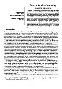
discussed in detail in the methods section, but is basically a linear inversion of the electrostatic forward solution and includes the boundary points. Evoking LFPs in the STN requires stimulation of pre-synaptic neuronal populations. Anatomical tracing studies in rodents show that the STN receives direct afferent input from the cortex (Figure 1) and from the globus pallidus externa (GPe) (Janssen et al. 2010; Bevan et al. 1995; Kolomiets et al. 2001; Hamani et al. 2004). The GPeSTN projection is part of the corticobasal ganglia-thalamo-cortical loop and STN-GPe-STN feedback loop (Figure 2). Figure 2, A schematic view of the mono-synaptic cortico-STN The different synaptic pathways will pathway, the mono-synaptic GPe-STN pathway, and the place of the have its influence on cortex stimulated GPe-STN pathway in the cortico-basal ganglia-thalamo-cortical loop and STN-GPe-STN feedback loop. White arrows denote excitatory evoked LFPs in the STN. Previous projections and blue arrows inhibitory projections. The STN, GPe, electrophysiological studies, show a striatum and pallidum are all part of the basal ganglia. (Figure modified from (Nambu et al. 2002)) typical multiphasic response in the STN after motor cortex (MC) stimulation, i.e. an initial excitatory response, interrupted by a short inhibition period, followed by a long inhibitory period (Figure 3A)(Fujimoto & Kita 1993; Magill et al. 2004; Kolomiets et al. 2001). It is believed that the typical profile is a result of the different pathways. Magill et al. (2004) suggests that the first peak N1 is due to activation of the monosynaptic MC-STN

Figure 3, A typical multiphasic profile of the motor-cortical stimulation-evoked LFP found in rats (A). N1, is probably due to activation of the monosynaptic MC-STN pathway (B). The short-latency, positive deflection, P1, probably arose as a consequence of feed-forward excitation of GPe(C). The long-latency, negative deflection, N2, was most likely due to disinhibition of STN through inhibition of GPe by the striatum, called the indirect pathway (D). The cause of P2 is unknown but thought to be caused by cortical disfacilitation. Figure by (Magill et al. 2004)

9

pathway (Figure 3B). The short-latency, positive deflection, P1, probably arose as a consequence of feed-forward excitation of globus pallidus (Figure 3C). The long-latency, negative deflection, N2, is most likely due to disinhibition of STN through inhibition of GPe by the striatum, called the indirect pathway (Figure 3D). The cause of the last positive deflection P2 is unknown but is thought to be caused by cortical disfacilitation. The temporal behavior of the LFP response would not be of any interest for electrophysiological mapping if there was not any spatial variation in the distribution. Fujimoto et al. (1993) found that in the peripheral part of the STN tend to lack the brief inhibitory component and exhibit a long period of excitation. Magill et al. (2004) found that the typical multiphasic LFP response was not seen in the caudal half of the STN. Besides, they also found that by reducing the stimulus strength it is possible to reduce the influence of the longer latency responses, i.e. N2 and P2 tends to disappear. Especially N2 is thought to be related to the polysynaptic pathway. Therefore, variation of the stimulation strength will cause variation of the distribution in case of spatial deviation between the monosynaptic and polysynaptic input. The only way to improve the electrophysiological mapping is by finding unique spatial restricted properties within the STN. Our goal in this study is finding these properties and will do this in an experimental setup in a rat model. In a systematic procedure cortex evoked LFPs are measured on 320 different locations within the rat STN. Instead of using the LFP in the electrophysiological mapping, we use the LFP to construct the CSD by using the iCSD method as described by Łęski et al. (2007). The CSD is used to describe the evoked synaptic activation within the STN. We expect spatial restricted properties in the evoked synaptic activation, because we activate different synaptic pathways. We can distinguish between the monosynaptic and polysynaptic pathways. The monosynaptic pathways from the cortex show a functional topology within the STN (Figure 1). Therefore, we will electro stimulate two cortex areas with different functions. Namely, the MC and the cingulate gyrus (CG) a cortex area evolved in the limbic system. The CG will most likely have a response located in the medial part of the STN, while evoked activation in the MC will have a response located in the dorsal part of the STN. The influence of the polysynaptic pathway on the MC evoked LFP is seen in the typical multiphasic LFP profile (Figure 3). We will use the timing of the positive and negative deflections in the MC evoked LFP to investigate spatial behavior of the synaptic activation (Sources/Sinks) in the CSD. Besides, we use two stimulation intensities for MC stimulation to vary the influence of the polysynaptic input. Taken together, we will relate the spatial behavior of the evoked sources and sinks in the CSD to the different neural pathways and the functional areas in the STN, and subsequently discuss the possibility to use the sources and sinks for localization within the STN.

10

4. Materials and methods 4.1 Experimental methods All animal experiments were carried out at the Université Victor Segalen Bordeaux 2 (Bordeaux, France) by Mark Janssen.

4.1.1 Animals Experiments were carried out on male Sprague Dawley rats (IFFA Credo) weighing 250-400 g. All experiments were done in accordance with the guidelines for the care and use of laboratory animals of the European Economic Community (86-6091 EEC) and the French National Committee (décret 87/848, Ministère de l Ag i ultu e et de la Fo êt , and were approved by the Ethical Committee of Centre National de la Recherche Scientifique, Région Aquitaine-Limousin. In total, 19 rats were used for the electrophysiological recordings, from which four rats were used for pilot experiments to optimize the stimulation and recording parameters.

4.1.2 Recording setup The rats were anesthetized with urethane hydrochloride (1.2 g/kg i.p. injections, Sigma-Alrich, France) and fixed in a stereotaxic apparatus (Horsley Clarke apparatus, Unimécanique, Epinay sur Seine, France). Body temperature was monitored with a rectal probe and maintained at 37 °C with a homeothermic warming blanket (model 50-7061, Harvard Apparatus, Les Ulis, France). Burr holes were made above the stimulation and recording sites. A saline solution was applied on all exposed cortical areas to prevent dehydration. A 10 mm long probe with 16 iridium contacts (30 µmm diameter - 703 µm2 contact area) and 100 µm intercontact distance (A1x16–10mm–100–703–A16 , Neuronexus, Ann Arbor, USA) was used for unit activity and LFP measurements (Figure 4). The recording electrode was slowly lowered into the brain using a motorized drive at the following position relative to Bregma (in mm): AP -2.8, ML -2, DV -8.2 (G Paxinos & Watson 1998); the deepest contact was Figure 4, The Neuronexus measurement positioned ventral to STN. To this aim the neuronal unit electrode: A1x16–10mm–100–703–A16. The electrode configuration has a 10 activity was monitored online. From the first trajectory (AP - mm long probe with 16 iridium contacts 2 3.8, ML -2.5) the recording electrode was repositioned (30 µm diameter - 703 µm contact area) and 100 µm intercontact distance. according to the Paxinos and Watson atlas in the medio-lateral and anterio-posterior plane at the same ventro-dorsal level to acquire neural responses in all STN subareas (see measurement protocol). LFP and unit recordings were done simultaneously. With a sample frequency of 1.395 kHz for the LFP and 22.32 kHZ for the unit recordings. The raw signal was amplified and filtered to extract the LFP and spike data using the AlphaLab SnR setup (AlphaOmega, Jerusalem, Israel). To obtain the LFP data the raw signal was low-pass filtered between DC and 357.1 Hz and the spike data was obtained after high-pass filtering (357.1 Hz). As reference a crocodile clamp was placed on the skin around the burr hole.

11

4.1.3 Electrical stimulation of the prefrontal cortices A construction of two homemade, concentric bipolar electrodes was used for stimulation of two cortical regions ipsilateral to the recording site, namely the MC and the CG (Tan et al. 2010). Stereotactic coordinates relative to Bregma were (in mm): AP 3.2, ML 4.0, VD 2.6 and respectively ML 0.8, VD, 2.6 (Paxinos and Watson 1998). Electrical stimuli were generated with an isolated stimulator (DS3, Digitimer Ltd., Hertfordshire, UK) triggered by the AlphaLab SnR (AlphaOmega, Jerusalem, Israel). Stimulation consisted of 99 monophasic pulses of 0.6 ms width and 300 or 600 μA intensity delivered at a frequency of 1.1 Hz (to avoid synchronization of 50Hz). At the beginning of each stimulus, a digital event was stored in the acquired signal.

4.1.4 Measurement protocol The experiment started by lowering the 16 channel laminar electrode within the STN. When the electrode was at its final position the recordings started. The first recording session was a baseline recording, the second and third recording sessions were MC stimulation sessions and the fourth recording session the CG stimulation session. We used two different stimulation protocols in the MC stimulation sessions, namely the 300 μA and 600 μA intensity pulse stimulation. The CG stimulation session only used the stimulation protocol with the 600 μA intensity pulse. After the four recording sessions, the measurement electrode was retrieved and inserted back into the brain, but shifted 200 micrometers along the anterior-posterior and/or medial-lateral axis direction. The electrode was placed at exactly the same depth as during the previous session and the four recording steps were then repeated on the new location. In total, the electrode was shifted 20 times, providing a 4x5

Figure 5, shows a rat brain with 4 subsequent coronal slices. The four pictures below show a zoom in on the coronal slices with the STN denoted in grey. The location of the measurement electrodes are denoted by the 320 black dots in the 4 slices. The 4x5x16 electrode positions together form the 3D measurement grid.

12

measurement grid (anterior-posterior x medial-lateral). Together with the depth measurements along the dorsal-ventral axis, provided by the 16 contact points of the recording electrode, a 3D measurement grid of 4x5x16 (anterior-posterior x medial-lateral x dorsal-ventral) was obtained (Figure 5). However, after each individual stimulus we only measured the evoked response on 16 different locations and not on all the 320 (4x5x16) measurement points. By taking the mean response in time for the 99 stimulations, we believed the temporal deviation introduced by the consecutive measurements is minimized. This allowed us to interpret the 3D measurement grid filled with the mean responses as if the response was simultaneous measured on 320 different points. To do so, we kept the reference and stimulation electrode fixed at the exact same location throughout the entire experiment.

4.1.5 Histology Before the electrode was lowered into the brain it was dipped in a red fluorescent dye: 1,1'Dilinoleyl-3,3,3',3'-Tet a eth li do a o a i e Pe hlo ate FA“T DiI™ oil; DiIΔ9,12-C18(3), ClO4). After the experiments animals were sacrificed, brains were collected and frozen in isopentane at -45°C and stored at -80°C. Fresh-frozen brains were cryostat-cut on glass into coronal sections for localization of stimulation track in the cortex and STN. Sections were examined under a microscope (Olympus AX70) to verify the electrode trajectories and tip positions of the different measurements. The trajectories were drawn in a rat brain atlas (G Paxinos & Watson 1998) and photographs of the trajectories were made using a camera (Olympus DP70) mounted on the microscope (Tan et al. 2011).

4.2 Data analysis The recorded data was divided online in high frequency spike data and low frequency LFP data. The LFP and spike data for the four recording sessions resulted in 8 different data sets for each of the 320 (4x5x16) measuring points. The main focus in this study was on the LFP recordings, but the spike recordings were used for validation. All the data was stored and processed offline in Matlab R2011b (Mathworks, Natick, USA).

4.2.1 Spike histogram

analysis:

peristimulus

time

The spike data was used to create Peristimulus time histograms (PSTHs). PSTHs are histograms of the times at which neurons fire. These histograms are used to visualize the rate and timing of neuronal spike discharges in relation to an external stimulus. PSTHs were generated by using an envelope spike detection method (Dolan et al. 2009). The high frequency spike data were visually examined to observe the spike threshold levels. Peaks above the threshold were marked as spikes and the waveforms of the detected spikes were used to classify the neurons (Lewicki 1998). The classification was performed by principal component analysis on the found waveforms. The first and second principal components were used for clustering. We

Figure 6, The typical MC evoked multiphasic response found in the PSTH and LFP in the STN. The timing of the negative deflection N1 correspond to the first excitatory phase in PSTH, The first positive deflection P1 to the first short inhibitory phase and P2 to the start of the long inhibitory phase (modified from Magill et al. (2004)).

13

used a Bayesian clustering, which used a probability density function (Gaussian mixture model) and expectation maximization. Finally, the spikes were binned with a binsize of 1 ms and the mean amount of binned spikes around stimulation was plotted in a time span from 10 ms pre stimulus to 60 ms post stimulus. The PSTHs were solely used as a validation method. Unit activation in the STN evoked by motor cortical stimulation shows a typical response in the PSTHs (Kolomiets et al. 2001; Fujimoto & Kita 1993; Magill et al. 2004). Magill et al. (2004) also showed a direct relationship between the PSTHs and LFPs measured in the STN after MC stimulation. In each experiment we examined the LFPs (see next section) and PSTHs after MC stimulation to find the same responses as described by Magill et al. (Figure 6). The finding of the multiphasic response confirmed that a part of the STN was within the measurement grid, the stimulation electrode evoked a response and the measurement setup measured relevant LFPs. The case in which we did not find the complete multiphasic response (including N1, P1, N1 and P2) in any of the 320 measurement points we excluded the rat from further analyses. After the validation procedure, we created for the remaining rats the CG evoked PSTH and LFP in the same manner as we did for the MC evoked measurement.

4.2.2 LFP analysis: Pre-processing All LFPS were filtered by a zero-phase digital high-pass filter to remove low frequency drift in the LFPs. A second order high-pass Butterworth filter with a 2 Hz cutoff frequency is used in the forward and reverse direction on the data(Oppenheim & Schafer 1989). This resulted in a fourth order highpass Butterworth filter with zero-phase distortion. The power spectral density of the LFP baseline for each of the 320 measuring points was estimated using Welch method. The data was split into 8 equal length overlapping segments with 50% overlap. Each segment was windowed with a Hamming window that was the same length as the segment. The segments were used to compute 8 periodograms, which were then used to produce the power spectral density (PSD) estimate. The PSD was numerical integrated between 2 and 357 Hz to find the signal power. Channels with power 10 times above average were considered to be artifacts and excluded from further analysis. To restore the 3D measurement grid we filled up the gap by 3D linear interpolation. After the baseline analysis, we processed the evoked LFP data. First, the epochs were examined (visual inspection) and epochs with artifact were excluded from further analysis. Next, the recordings were stimulus averaged (99 epochs) and smoothed over time with a Savitsky–Golay filter. The filter performed a third order polynomial regression within a 9 sample window by minimizing the least square error. The main advantage of the Savitsky–Golay filter over a moving average filter was that it preserved features as relative maxima, minima and peak width (Savitzky & Golay 1964). Finally, the 3D measurement grid was spatially smoothed in dorsal-ventral direction by a Savitsky–Golay filter. We also used a third order polynomial regression, but used a smaller window size (5 samples), because we had only 16 points in the dorsal-ventral direction.

14

4.2.3 LFP analysis: Signal normalization As explained in the measurement protocol, we interpreted the measurement data as if it was simultaneous measured in a 3D grid. This assumption seemed fair but might be corrupted when the measurement electrode get damaged or soiled during the measurement process. This would influence the electrode impedance and as it was impossible to have an amplifier with infinite input impedance it would influence the amplification of the measured signals. To counter this we looked at several methods for normalization (Power/RMS/artifact height) of the LFP data as explained in Appendix A. The root mean square (RMS) normalization was used in the further analyzes. The RMS of the signal described the deviation of the signal. The deviation was a function of the amplifier gain, i.e. higher gain resulted in more deviation. Therefore, the RMS could be used in the normalization. However, the RMS was also a function of the activity of the local neuronal populations. As previously explained, we expected different LFP responses on different locations and therefore also a distribution of different RMS values. We wanted to keep this information. Therefore, to reduce the influence of the local neuronal populations on the RMS normalization, we used for each physical electrode the mean RMS value over all rats, different locations and different stimulation protocols. In detail, for each experiment which showed the multiphasic MC response in the LFP, we calculated the RMS values of the average MC and CG evoked LFP responses. This gave 320 RMS values for each measurement session from which 20 were recorded with the same physical electrode. Next, the mean RMS was calculated for each electrode and for each measurement session these mean RMS values were normalized by dividing them by the maximum mean RMS of that session. Finally, the mean RMS value over all measurement sessions was calculated by taking the mean of each normalized mean RMS value. The RMS normalization was done before the spatial filtering. All the recordings for each of the 16 physical electrodes were multiplied by their mean RMS value and divided by the maximum mean RMS value.

4.2.4 LFP analysis: Inverse Current Source Density The extracellular potential was generated by currents crossing the cell membranes and a standard method to analyze LFP s as to estimate this CSD. By using the CSD to describe the neural activity it was possible to achieve higher spatial resolution. The general approach to calculate the CSD was to use the static approximation of the electrodynamics equations and assuming the extracellular medium to act as an ohmic volume conductor in the relevant frequency range [Equation 1]. ∇ · (σ∇LFP) = −CSD

[1]

With LFP the local field potential [V], σ the electrical conductivity tensor [Ω-1m3] and CSD the current source density [I/m3]. In general, the electrical conductivity tensor was anisotropic and depended on position. However, in the traditional CSD method the conductivity was assumed to be a constant scalar, because the conductivity properties were unknown. In this case, the CSD was the second order derivative of the LFP and could be estimated by a numerical estimation of the Laplacian operator. The main drawback of a numerical derivative was the exclusion of all the boundary points. In a 3D grid, a significant amount of the measurement points were boundary points and exclusion of all these points was unacceptable. For example, in the 3D grid we used in this study, there were 236 boundary points out of the 320 total points (4 x 5 x 16). Another approach to estimate the CSD was called the inverse Current Source Density (iCSD) method and was described for one dimensional 15

recordings by Pettersen et al. (2006) and generalized to three-dimensional recordings by Łęski et al. (2007). In this procedure, the CSD was assumed to have a certain known distribution class. This distribution class needed to be parameterized with as many parameters as the number of recorded signals. By using the electrostatic forward solution on the known CSD distribution, one can find a linear relation, described by linear transformation matrix F, between the parameters of the CSD distribution and the LFPs generated by the CSD on the electrode locations [Equation 2]. The linear relation was used to solve the inverse problem by using the inverse of F to calculate the CSD parameters from the recorded LFP signals [Equation 3]. =

=

With the LFP vector ( ), the CSD vector ( ) and the iCSD transformation matrix. The LFP vector consisted of 320 potentials corresponding to the measured LFP on the electrode positions after a given time post stimuli. The CSD vector consisted of the 320 CSD parameters. The CSD parameters described a CSD distribution of a certain class. Different classes can be defined; in appendix B we showed a basic example. In this study, we used a more sophisticated class called natural spline iCSD in which the CSD values on the measurement grid were used as parameters and the CSD values within the grid were obtained using natural spline interpolation. Łęski et al. (2007) described one iCSD drawback and a solution for this problem. The iCSD method assumed all the current sources within the measurement grid. This assumption leads to errors at the boundaries in case there were sources outside the measurement area. This was because the iCSD method tried to imitate the influence of these sources by adjusting the source density at the boundaries. This error was reduced by extending the CSD distribution with one layer beyond the original grid and duplicate the nearest CSD value for these points (D boundary conditions). Summarizing, we used a natural spline iCSD method with D boundary conditions to convert the measured LFPs into the CSD.

4.2.5 CSD analysis: Significant Sources and Sinks For each individual rat, the 320 LFP baseline recordings were used to find the baseline CSD distribution. To create the baseline CSD, we treated the baseline LFP exactly the same as the evoked LFPs. This means, the baseline data was high pass filtered on 2 Hz and was split in 99 segments. Finally, the mean was taken over the 99 segments, RMS normalized and filtered (spatially/temporally). This resulted in a mean LFP baseline grid which we used to calculate the baseline CSD grid by using the natural spline iCSD method with D boundary conditions. The mean and standard deviation (std) of the values in the CSD baseline grid was compared with the evoked CSD values. We assumed a normal distribution of the data. With this assumption, the evoked CSD on a certain time was statistically significant (significance level α=1%) when it was higher or lower than the baseline mean ± n (n = 2.58) times the baseline std [Equation 4]. =

−

With α the significance level, erf the error function and n the deviation in units of the std.

16

4.2.6 CSD analysis: Visualization The rat atlas (G Paxinos & Watson 1998) was used for the visualization of the STN. The location of the electrode in anterior-posterior and medial-lateral direction was based on the stereotaxic coordinate given by the stereotaxic apparatus. The neuronal unit activity was monitored online to place the deepest contact ventral to the STN. Therefore, we did not use the ventral-dorsal stereotaxic coordinate but located the deepest electrode ventral to the STN in the visualization. In the CSD, only the significant sources and sinks were plotted. The outflow of negative charged ions or inflow of positive charged ions in the extracellular medium will cause sources in the CSD and are denoted in a red color scale. The outflow of positive charged ions or inflow of negative charged ions in the extracellular medium will cause sinks in the CSD and are denoted in blue color scale (Pettersen et al. 2008). The non significant sources and sinks are plotted in green. For each rat the CSD was constructed at the time of the negative deflection N1 and the positive deflections P1 and P2 for that individual rat.

17

18

5. Results 5.1 Histology The red fluorescent dye was diffused through the tissue and was therefore impossible to use for tracking the individual electrode trajectories. However, by looking at the deformation of the tissue, we were able to track the electrode trajectories (Figure 7). The brains from the first 5 rats were not cut and plated and the brain from rat #8 was too damaged in the cutting procedure to trace the trajectories. In rat #7 we found electrode trajectories near STN (bregma -3.3 mm) but did not have slices beyond bregma -3.3 mm, therefore we were not able to find trajectories into STN. In the other 12 rat brains, we found trajectories within the STN, with the deepest electrode down to the ventral part of the STN.

5.2 Multiphasic MC Response: PSTH and LFP. The multiphasic MC response, including the long and short latency phase (N1, N2 and P2) in the PSTH and LFP was found in rat #5, #7, #9 and #11 (Figure. 8). The remaining rats did not show the complete multiphasic response and were excluded in further analysis. In the evoked LFP and spike measurements we noticed a wide stimulation artifact (6 ms), therefore we did not plot the first 6 ms after stimulation in the PSTH. The peak of the 6 ms wide stimulation artifact in the measured LFP was 3 ms after beginning of the stimulation.

Figure 7, (A) A selection of a microscope picture of a coronal brain slice (Rat #16, Anterior-posterior -3.8 mm relative to Bregma). The STN (B) and electrode trajectories (C) can be seen in the brain slice.

In total we measured 50 multiphasic LFP responses after MC stimulation with intensity 600 µA and three multiphasic LFP responses after MC stimulation with intensity 300 µA. On average, the first negative deflection N1 occurred at 9.5s±0.9 ms, the first positive deflection P1 occurred at 14.5±1.9 ms, and the second positive deflection P2 occurred at 32.2±2.6 ms. See table 1 for latency values per rat. Rat #7 and #11 showed a slightly faster response then rat #5 and #9.

19

Figure 8, examples of LFP and PSTH multiphasic reponses in rat #5, #7, #9 and #11. The evoked response is caused by MC stimulation with stimulation intensity 600 µA on t=0. The negative deflection , N1, and the two positive deflections P1 and P2 can be seen in each of the four rats.

Figure 9, examples of LFP and PSTH multiphasic reponses in rat #5, #7, #9 and #11. The evoked response is caused by CG stimulation with stimulation intensity 600 µA on t=0. The negative deflection , N1, and the two positive deflections P1 and P2 can be seen in rat #5, #9 and # 11. In rat #7 we did not find a response with clear negative and positive deflections.

20

Rat

Number of Mean N1 (ms) Reponses Latency values individual rats (MC stimulation): #5 12 10.73 ± 0.33 #7 23 8.63 ± 0.28 #9 12 9.89 ± 0.37 #11 6 9.60 ± 0.29 Average latency values (MC stimulation): 53 9.5 ± 0.9 Latency values individual rats (CG stimulation): #5 7 15.21 ± 0.59 #7 0 #9 30 11.75 ± 0.42 #11 19 11.82 ± 0.52 #5 7 15.21 ± 0.59 Average latency values (CG stimulation): 56 12.2 ± 1.24 Difference between CG and MC stimulation: +2.7

Mean P1 (ms)

Mean P2 (ms)

16.76 ± 0.67 12.7 ± 0.57 15.99 ± 0.89 13.54 ± 0.58

35.77 ± 0.99 30.26 ± 1.43 33.43 ± 0.71 30.38 ± 1.46

14.5 ± 1.9

32.2 ± 2.6

19.61 ± 0.49 16.95 ± 0.96 16.95 ± 0.97 19.61 ± 0.49

36.31 ± 0.70 34.95 ± 1.66 36.49 ± 2.15 36.31 ± 0.70

17.28 ± 1.27

35.64 ± 1.9

+2.8

+3.4

Table 1, Latency values (± STD) for the evoked negative and positive deflections in the LFP after stimulation.

5.3 Multiphasic CG response: PSTH and LFP. The CG stimulation also caused a multiphasic response in the PSTH and LFP in rat #5, #9 and #11. However, Rat #7 did not show a clear response to the CG stimulation (Figure. 9). Also in the CG evoked LFP and spike measurements we noticed a wide stimulation artifact (6 ms), therefore we did not plot the first 6 ms after stimulation in the PSTH. The peak of the 6 ms wide stimulation artifact was at 3 ms after beginning of the stimulation. In total, we measured 56 multiphasic LFP responses after CG stimulation. On average, the first negative deflection N1 occurred at 12.2±1.24 ms, the first positive deflection P1 occurred at 17.28±1.27 ms, and the second positive deflection P2 occurred at 35.64±1.9 ms. See table 1 for latency values per individual rat. Comparing CG to MC stimulation the latency values are on average higher (N1= 2.7 ms higher, P1 = 2.8 ms higher, P2= 3.4 ms higher).

21

5.4 Spatial distribution of MC evoked LFP The MC evoked LFP responses in rat #5, #7, #9 and #11 showed spatial deviation. The previously described multiphasic MC response was best seen with stimulation intensity 600 µA. Of the 320 measured responses only a few showed peak P2 clearly in the multiphasic response. These responses were located in the lateral-rostal part of the STN. While P2 was only seen in a small part of the STN, P1 was found through the whole STN. Finally, N1 was best seen medially of the multiphasic responses including P2 (Figure 10). In comparison to the MC stimulation with intensity 600 µA, the MC stimulation with intensity 300 µA showed a reduction of peak P2 in the evoked responses. A spatial deviation of N1 was still seen in the evoked responses (Figure 10)

Figure 10, A coronal view of the rat STN (G Paxinos & Watson 1998) (coronal distance = -3.6 mm relative to Bregma). Within the boxes the MC evoked responses in rat #9 are plotted. The black point in the box denotes the measurement electrode location. The black arrows denotes the time of stimulation. (A) The left view shows the spatial behavior of the MC (600 µA) evoked response. The multiphasic response within the red box shows the positive deflection P2 clearly. The multiphasic response within the green box shows the negative deflection N1 clearly. (B) The right view shows the spatial behavior of the MC (300 µA) evoked response. Positive deflection P2 is not measured, but the negative deflection N1 is seen clearly in the green box.

22

5.5 Spatial distribution of CG evoked LFP The CG evoked LFP responses in rat #7 showed no spatial deviation. That is, we found no CG evoked response in rat #7. Therefore, we were not able to analyze the spatial behavior of the response. We did find CG evoked multiphasic LFP responses in rat #5, #9 and #11 which showed spatial deviation. However, the spatial behavior was not consistent for the three rats. Rat #5 showed the multiphasic CG responses on the same location as the multiphasic MC responses. In rat #9 and #11 the multiphasic CG responses were 0.1 mm more medial-ventral located of the multiphasic MC responses (Figure 11).

5.6 Spatial distribution of MC evoked CSD For rat #5, #7, #9 and #11, we created CSD Figure 11, a coronal view of the rat STN (G Paxinos & Watson plots by using the spline iCSD method with 1998) (coronal distance = -3.6 mm relative to Bregma). Within duplicate boundary conditions. For each the boxes the in rat #9 CG evoked responses are plotted. The block point in the box denotes the measurement electrode rat, we focused on the CSD around the time location. The black arrows denotes the time of stimulation. The of N1, P1 and P2 of that individual rat (table different boxes show the spatial behavior of the CG (600 µA) 1). Even after the RMS normalization and evoked response. The mulitphasic response (for example the red box) are located in the medial ventral part of the STN. smoothening of the LFP data in ventraldorsal direction we noticed alternating laminar patterns in the CSD. Nevertheless, we found typical spatial behavior of the sources and sinks in the CSD after MC stimulation. After MC stimulation with intensity 600 µA, a significant sink appears on t≈N1 and lateral of this sink a significant source appears on t≈P2 (Figure 12). After MC stimulation with intensity 300 µA the same but weaker significant sink appears on t≈N1. In rat #9, we also find a weak source on t≈P2, but in the other three rats it were impossible to distinguish the source on t≈P2 (Figure 12). We did not find any consistent spatial behavior of the sources and sinks around t≈P1.

23

A

B

Figure 12, Example (rat #9) of the evoked significant sources (red/yellow), sinks (blue) and no significant sources (green) in the CSD. The CSD is created using a spline iCSD with duplicate boundary conditions. (A) After MC stimulation with intensity 600 µA there is a sink at AP:-3.6mm, ML: 2.5mm, VD:-7.75mm (relative to Bregma) on t=10.2 ms (=N1). No clear source/sink is seen at t=15.9 ms (=P1) and a clear source is seen at AP:-3.6mm, ML: 2.6mm, VD:-7.8mm (relative to Bregma) on t=33.1 ms (=P2). (B) After MC stimulation with intensity 600 µA there is a sink at AP:-3.6mm, ML: 2.5mm, VD:-7.8mm (relative to Bregma) on t=10.2 ms (=N1). No clear source/sink is seen at t=15.9 ms (=P1) and a small source is seen at AP:-3.6mm, ML: 2.6mm, VD:-7.8mm (relative to Bregma) on t=33.1 ms (=P2).

24

5.7 Spatial distribution of CG evoked CSD In our evaluation of the CSD after CG stimulation, we focused around the time of N1, P1 and P2 of that individual rat (table 2). Even after the RMS normalization and spatial smoothening of the LFP data in ventral-dorsal direction, we noticed alternating laminar patterns in the CG stimulated data. We did not find any consistent spatial behavior of the sources and sinks in the evoked CSD. In general, we saw many different sources and sinks in and outside the STN.

Figure 13, Example (rat #9) of the evoked significant sources (red/yellow), sinks (blue) and no significant sources (green) in the CSD. The CSD is created using a spline iCSD with duplicate boundary conditions. After CG stimulation with intensity 600 µA there is significant activation seen within the STN and in the tissue above. But we did not find any consistent spatial behavior of the sources and sinks in the CG evoked CSD.

25

26

6. Discussion 6.1 Data validation In this study we used an innovative data analyses method, the iCSD method, to describe the neuronal activity within the STN. Because of the novelty of the analyses methods we used a strict validation procedure to make sure there were no errors in the data set. The validation procedure of the electrophysiological signals consisted of finding the MC evoked multiphasic response as described in literature (Kolomiets et al. 2001; Fujimoto & Kita 1993; Magill et al. 2004). The fact that we measured this typical multiphasic response in the LFP as well as in the PSTH in rat #5, #7, #9 and #11 showed that for these rats at least a part of the STN was within the measurement grid, the stimulation electrode evoked a response and the easu e e t setup easu ed ele a t LFP s Figu e . The disadvantage of the strict validation procedure was that we ended up with four of the 19 rats for further analyses. The first four of the 19 rats were only used for pilot experiments to optimize the stimulation and recording parameters. In the 11 remaining rats, we did not measure the MC evoked multiphasic response. There are different possibilities why we did not find any evoked multiphasic response in the 11 rats. The first possibility is that we measured on the wrong location. That is, none of the 320 measurement points of the 3D measurements grid were located in the dorsal-rostal part of the STN. However, a histology validation showed that we did measure within the STN for 12 of the 14 histology prepared rats (Figure 7). The second possibility is that the cortex stimulator was stimulating in the wrong area or stimulating too weak to evoke a response in the STN. We looked explicitly to P2, the last positive deflection in the evoked LFP, in our decision to exclude the rat for further analyses. Magill et al. (2004) showed that P2 disappears with a reduction of stimulation intensity. However, they still found P2 with a stimulation intensity of 300 µA while we did not even find P2 after stimulation with intensity of 600 µA in the 11 remaining rats. Finally, the third possibility is that the signal to noise ratio was too low and that we could therefore not distinguish the evoked response from the noise. The four rats in which we found the evoked responses were all in the first half of the 15 rat experiments (19 rats minus the 4 pilot experiments). Rat #11 was the last rat which showed a multiphasic MC response including P2. Comparing the measured P2 from the last rat (rat #11) with the P2 from the first rat (rat #5) we see that P2 from rat #11 is less clear (Figure 8). This might indicate a decrease of the signal to noise ratio over the experiments. In addition, we used one measurement electrode for all 19 experiments. So, the decrease of signal to noise ratio might be caused by wear of the measuring electrode. This last possibility was most likely the reason we did not find an evoked response in each experiment, but we were not able to verify this.

6.2 Evoked LFP’s in the STN In the four rats, we found 53 MC evoked multiphasic responses that included P2. In these responses, we found an average latency of 9.5±0.9 ms for N1, 14.5±1.9 ms for P1 and 32.2±2.6 ms for P2. Magill et al. (2004) found in similar experiments an average latency of 5.4±1.3 ms for N1, 11.9±2.8 ms for P1 and 30.7±5.3 ms for P2. The difference between the latencies is probably due to a different definition of t=0. In our experiment we defined the start of stimulation as t=0. In the case, we take the peak of the stimulation artifact as t=0 we get an average latency of 6.5±0.9 ms for N1, 11.5±1.9 ms for P1 and 29.2±2.6 ms for P2, which are all within the deviation of the latencies found by Magill et al. (2004).

27

We also found 56 CG evoked multiphasic responses included P2. In these responses, we found an average latency of 12.2±1.24 ms for N1, 17.28±1.27 ms for P1 and 35.64±1.9 ms for P2. Comparing CG to MC stimulation the latency values are on average higher (N1= 2.7 ms higher, P1 = 2.8 ms higher, P2= 3.4 ms higher). This indicates that the CG-STN pathway is longer than the MC-STN pathway. The STN-GP-STN feedback loop, that is the difference between N1 and P1, seems to be of the same length for both systems.

6.3 Localization of the electrodes and visualization of the data The goal of the study was to find unique spatial properties of the evoked electrophysiological signals in the STN. To do spatial analyses, we had to know the location of the STN within the 3D measurement grid. For this purpose, we used the stereotactic location of the electrode and a rat atlas for the visualization of the STN. The rat atlas was developed by study of medium-sized (average 290 g) male Wistar rats. However, no substantial stereotaxic error will occur when rats of different sex and strain are chosen, provided that the rats are of similar weight to those on which the atlas is based. In our study, we used Sprague Dawley rats (IFFA Credo) weighing 250-400 g. Nevertheless in most cases, the position of a brain structure is represented in the atlas to an accuracy of less than 0.5 mm (G Paxinos & Watson 1998). For a small brain structure like the STN a deviation of only 0.5 mm is still significant. Therefore, we did a histology validation. The red fluorescent dye was diffused through the tissue and was therefore impossible to use for tracking the individual electrode trajectories. We were able to use the deformation of the tissue to track the electrode trajectories, but were not able to track down each electrode for each rat. Nevertheless, we found in 12 of the 14 histology prepared brains the electrode trajectories within the STN with the deepest electrode down to the ventral part of the STN. This indicates that the stereotactic coordinates in combination with the rat atlas can be used for the visualization of the measured data.

6.4 The iCSD method To create the CSD, we used 3D spline iCSD with duplicate boundary conditions Łęski et al. ; Pettersen et al. 2006). Łęski et al. (2007) showed that the iCSD method had a main drawback; the method assumed all the current sources within the measurement grid. This assumption leads to errors at the boundaries if there are sources outside the measurement area, because the iCSD method tried to imitate the influence of these sources by adjusting the source density at the boundaries. This error is reduced by extending the CSD distribution with one layer beyond the original grid and duplicates the nearest CSD value for these points. This proposed method gave a sufficient reduction of the boundary artifacts in our study. Another drawback of the spline iCSD method is the sensitivity to spatial noise (Pettersen et al. 2010). Therefore we performed RMS normalization and spatial filtering of the easu ed LFP s. Because of the low spatial resolution in the medial-lateral and anterior-posterior direction we decided to only filter in the dorsal-ventral direction. We used a Savitsky-Golay filter which performs a local 3rd order polynomial regression to determine the smoothed value for each point. In contrast to averaging techniques like moving averages, the Savitsky-Golay filter performs better in preserving features such as relative maxima, minima. The preserving of these features was important for finding the unique spatial properties in the evoked electrophysiological signals. However, even after filtering and normalization we still noticed artifacts.

28

6.5 MC evoked CSD In four rats, we found promising spatial and temporal deviation of the sources and sinks in the MC evoked CSD. After MC stimulation with intensity 600 µA, we found a strong localized sink in the STN at t≈N1. This was the time of synaptic activation through the excitatory hyper-direct (MC-STN) pathway (Magill et al. 2004). The localized sink indicates that the hyperdirect pathway only projects to a local part of the motor STN. This is not in agreement with anterograde tracing studies in rodents, the trajectory of the labeled fibers indicate that it is likely that individual cortical neurons innervate many subthalamic neurons over a large extend of the nucleus (Bevan et al. 1995). However, topographic organization is shown in electrophysiological studies (Kolomiets et al. 2001)(Nambu et al. 2000). These studies also use the multiphasic LFP and PSTH response, but no CSD analyses. The strong localized sink we found in the CSD shows that CSD analyses in a 3D measurement grid is an excellent tool to study topographic organized projections from the MC to the STN. After MC stimulation with intensity 600 µA, we also found a strong localized source at t≈P2. The positive deflection P2 in the LFP is at the start of the long inhibitory period seen in the STN spikes (Magill et al. 2004). The cause of P2 in the LFP is unknown, but it has been hypothesized to be caused by cortical disfacilitation (Fujimoto & Kita 1993). A reduction of the local excitatory input from the cortex in respect to the surrounding tissue might cause a source in the CSD. However, the source at t≈P2 was localized lateral to the sink we found at t≈N1. The displacement of the source with respect to the sink suggests that it is not caused by the same synaptic contacts. So more likely, the source was caused by a local inhibitory input. In the case of the STN, the only inhibitory projection is from Globus Pallidus externa (GPe), so through the indirect pathway. Cortical Figure 14. The top diagram shows the normal excitatory (exc) and inhibitory disfacilitation can be the cause of (inh) pathways between the cortex, striatum, globus pallidus externa (GPe) the inhibitory input from the GPe in and the subthalamic nucleus (STN). The bottom diagram shows the result of the following manner; the cortical disfacilitation; a decrease of excitatory input from the cortex (smaller arrows). This causes less excitation in STN through the hyperdirect excitatory projection from the pathway and less excitation of the striatum. Less activity in the striatum cortex to the striatum is reduced, results in less inhibition of the GPe (smaller arrow). This causes more which causes less inhibition of the inhibition of the STN through the indirect pathway (bigger arrow). GPe and results in more inhibition of the STN (Figure 14). After MC stimulation with intensity 300 µA we also found a localized sink in the STN at t≈N1, but weaker than the evoked sink after the 600 µA stimulus. This indicates that the STN receives less synaptic input from the MC. The reduction of stimulation intensity results in less activated neurons. 29

In our case, less activated neurons in the MC result in less synaptic activity in the STN, which is in agreement with our results. The difference between the CSD at t≈P2 after MC stimulation with intensity 600 µA and MC stimulation with intensity 300 µA is the strength of the source. In three of the four rats the source was not of significant strength. As noted before, the reduction of stimulation intensity results in less activated neurons. But the reduction of the stimulation strength seems to have a bigger influence on the source at t≈P2 than the sink at t≈N1. This indicates that the source and sink are caused by two different mechanisms. The sink is caused directly by the electro stimulation of the cortical neurons while the source is believed to be caused by cortical disfacilitation. Cortical disfacilitation is a form of inhibition during which neurons are hyperpolarized due to the temporal absence of excitatory synaptic activity (Timofeev et al. 2001). Most excitatory input to cortical pyramidal cells arises from thalamocortical neurons or other pyramidal cells, so the hyperpolarized state must arise from some influence that quiets these inputs (Wilson 2008). The whole cortical disfacilitation mechanism is not fully understood yet, but our result suggests it takes a higher electro stimulation intensity to quiet the excitatory inputs in the cortex then to evoke activation in the cortex. Another factor which may have an influence on the sink and source is that they are caused by different types of neurons in the cortex. For cats it was shown that the cortico-STN projections originate from the pyramidal tract type cells (Giuffrida et al. 1985), but this has not been confirmed in rats and monkeys. The axons projecting to the direct and indirect pathway presumably originate from intratelecenphalic type pyramidal cells in the MC (Ballion et al. 2008). The pyramidal tract neurons lay deeper in the cortex but have bigger axons which make them easier to innervate than the intratelecenphalic neurons. So this might explain why the sink at t≈N1 is still seen with lower stimulation intensity, but it might not be strong enough to cause disfacilitation in the intratelecenphalic cells.

6.6 CG evoked CSD We did not find any clear local sources in the CG evoked experiments. This can be caused by two possibilities. First, the synaptic input was localized but weak. Anterograde Tracing studies show a CGSTN projection but mainly MC synaptic input in the STN (Orieux et al. 2002; M. Bevan et al. 1995). This is in agreement with our results. When we compare between the MC and CG evoked PSTH and LFPs, we noticed a weaker LFP and less evoked spikes after CG stimulation (Figure 8 & 9). Second, the synaptic input was not topological organized and caused a global synaptic activation through the STN. However, to the best of our knowledge, there is no study which shows a difference between MC and CG synaptic segregation.

6.7 Clinical implications. The STN is an important electrode target in DBS therapy. Misplaced electrodes may induce unwanted stimulation related side effects (Krack et al. 2002; Tamma et al. 2002; Temel et al. 2006). It has been hypothesized that the adverse effects are caused by the fact that the STN incorporates three functional modalities, namely motor, limbic and associative functions. Consequently, stimulation of the areas that are not concerned with motor function results in adverse effects. Therefore, in the future the lo alizatio of the “TN s otor area should become an essential part of the electrode implantation procedure (Janssen et al. 2011; Temel et al. 2005). New stimulation electrode designs are able to both measure LFPs and selectively stimulate nearby areas (Martens et al. 2011). It would be a significant improvement when the stimulation electrode could be used to locate the motor-STN 30

through LFP measurements. Therefore we have to improve the electrophysiological mapping and the only way to improve the electrophysiological mapping is by finding unique spatially restricted properties within the STN. The strong localized sink at t≈N a d sou e at t≈P afte MC sti ulatio could act as ele t oph siologi al fi ge p i ts that might greatly aid in finding specific regions within the STN. However, our results are obtained from the rat model and not from the human STN. There are certain differences between the rat and human STN. First, the motor, limbic and associative subdivisions of the rat STN are not entirely segregated from each other (Janssen et al. 2012). The rat STN has a higher number of neurons per cubic millimeter (30,000 cells per mm3) compared to the human STN (2,300 cells per mm3) (Hardman et al. 2002) and the dendrites can extend across almost the entire STN (Heimer et al. 1995). Nevertheless, even with less segregation we found localized sources and sinks in the rat STN after MC stimulation. Second, the existence of the hyperdirect pathway is not proven in the human STN. If there is no hyperdirect pathway then there will be no localized sink at t=N1. This will be a loss for the electrophysiological mapping and reduces the localizing potential.

31

32

7. Conclusions and Recommendations In this study we showed an evaluation of evoked electrophysiological signals obtained in a 3D measurement grid within a rat STN. The 3D measurement grid proved to be a useful tool to analyze spatial deviation in the electrophysiological signals. In four rats, we found promising spatial and temporal deviation of the sources and sinks in the MC evoked CSD, which might be used for localization in clinical applications. The spatial behavior of the MC evoked sink at t=N1 and source at t=P2 indicates that they are caused by different synaptic pathways. The sink at t=N1 is evoked through the excitatory hyper-direct pathway while the source at t=P2 is evoked through the inhibitory indirect pathway. The variation of the MC evoked sink at t=N1 and source at t=P2 caused by variation of stimulation intensity suggests the response is caused by two different mechanisms. One mechanism is direct neuronal activation by electro stimulation the other mechanism might be cortical disfacilitation. In the future, the unique spatial en temporal behavior of the evoked CSD might be used as an electrophysiological map during DBS electrode placing. For future work and experiments, we have five recommendations: 1. It would be better to not use the rat atlas but visualize the sources and sinks on the actual STN of that rat. In our study, we were not able to do this, because we were not able to retrieve each electrode trajectory. One reason for this was the fluorescent dye diffused through the tissue; this could be overcome by perfusing the rats transcardially with paraformaldehyde. Instead of coloring each electrode trajectory, we commend to color one trajectory in each coronal cross section. And color a unique trajectory in lateral-medial direction for each coronal cross section. 2. Before each experiment there should be a calibration of the measurement setup. The calibration setup should notice wear of the electrode and changes in electrode impedances. This is important because of the sensitivity of the CSD method. 3. The iCSD method we used in this study performs well for local sources. In case of many spatially distributed sources and sinks we suggest to add independent component analyses for better results Łęski et al. . 4. The electrophysiological mapping in the clinic is mainly done by single unit recordings. For clinical purposes it would be interested to study the relation between the CSD and the single unit recordings. Because of the wide dendritic tree of the STN neurons it is not trivial that the single unit activity is also localized. Therefore we suggest to plot in Figure 10-11 not only the LFP but also the evoked PSTH. 5. In our validation method we decided to exclude all rats, which did not show the complete MC evoked multiphasic response. However, this does not mean that we measured irrelevant electrophysiological signals in excluded rats. Therefore we recommend to create and analyze the CSD for the excluded rats as well.

33

34

Appendix A: LFP Normalization In this study we created a 3D measurement grid by making 20 consecutive measurements with a 16 channel electrode on different locations within the STN. The signals measured on each location were 99 evoked responses within the STN after MC and CG stimulation. By taking the mean response in time for the 99 stimulations, we believed the temporal deviation introduced by the consecutive measurements is minimized. This allowed us to interpret the 3D measurement grid filled with the mean responses as if the response was simultaneous measured on 320 different points. This assumption seemed fair but might be corrupted when there are differences in electrode impedance. We found artifacts which can be explained by a difference in electrode impedances. The stimulation evoked CSD showed in several rats an extraordinary alternating pattern (Figure 15). The STN did not have a clear laminar structure like the cortex for example. However, the measurement electrode design showed a laminar alternating structure (Figure 15). All the sources (red) seemed to be on the right side of the electrode while the sinks (blue) seemed to be on the left side of the electrode. Therefore, we concluded this must be an electrode impedance artifact.

Figure 15, (A) The contour plot shows the reconstructed CSD for rat 9 around 15 ms post MC stimulation. The CSD showed an extraordinary alternating pattern. (B) The tip of the measurement electrode with each electrode number. (C) The sources in the CSD are measured on the right side of the connector, while the sinks are measured on the left side of the connector.

Normalization Methods To counter the electrode impedance artifacts, we looked at three different parameters for the normalization of the LFP recordings, namely, the power, the RMS and the height of the stimulation artifact. Each of these parameters had a relation with the electrode impedance, because the impedance affected the gain of the signal. When the gain was reduced also the power the RMS and the height of the stimulation artifact would be reduced.

RMS: For each evoked LFP measurement session, i.e. two MC evoked sessions (300 μA and 600 μA stimulation) and one CG session (600 μA stimulation) per rat, we calculated de RMS values for each measurement point. This gave 320 RMS values for each measurement session from which 20 were recorded with the same physical electrode. Next, the mean RMS was calculated for each electrode and for each measurement session these mean RMS values were normalized by dividing them by

Figure 16, The mean RMS values for each physical electrode over each measurement sessions ± STD.

35

the maximum mean RMS of that session. Finally, the mean RMS value over all measurement sessions was calculated by taking the mean of each normalized mean RMS value (Figure 16).

Power: For each evoked LFP measurement session, i.e. two MC evoked sessions (300 μA and 600 μA stimulation) and one CG session (600 μA stimulation) per rat, we calculated the power on each measurement point using Welch method. Welch method splits the data into 8 equal length overlapping segments with 50% overlap. Each segment was windowed with a Hamming window that was the same length as the segment. The segments were used to compute 8 periodograms, which were then used to produce the power spectral density (PSD) estimate. The PSD was numerical Figure 17, The mean power values for each physical integrated between 2 and 357 Hz to find the electrode over each measurement sessions ± STD. signal power. In each measurement session, we calculated the mean power for each of the 16 physical electrodes and divided it by the maximum power of that session. Finally, the mean values for each physical electrode over all measurement sessions were taken (Figure 17).

Stimulation artifact height: For each evoked LFP measurement session, we took the mean peak value of the 99 stimuli artifacts on each measurement point. This gave 320 peak values for each measurement session from which 20 were recorded with the same physical electrode. Next, the mean peak was calculated for each electrode and for each measurement session these mean peak values were normalized by dividing them by the maximum mean peak of that session. Finally, the mean artifact peak value over all measurement sessions was calculated by taking the mean of each normalized mean peak value (Figure 18.)

Figure 18, The mean artifact peak values for each physical electrode over each measurement sessions ± STD.

Conclusion Each of the three normalization variables had the same alternating structure as the artifacts we found in the CSD. Because of the high frequency character of the stimulation artifact in combination with the offline low-pass filtering on357.1 Hz and low sampling frequency of 1.395 kHz, we decided not to use the height of the stimulation artifact for normalization. The power and RMS show similar results, but because of computational time we decided to use the RMS values in our normalization.

36

Appendix B: Step-iCSD example The next example has the purpose to explain the idea of CSD classes and the modifications we did on the iCSD methods described by Łęski et al. (2007). The original iCSD method assumed a constant electrode distance in x, y and z direction. However, in our case the distance between the 16 electrodes in ventraldorsal direction was 0.1 mm but the distance in medial-lateral and anterior-posterior was 0.2 mm. We solved this by changing the Figure 19, An example CSD distribution. The measurement boundary conditions of the integrals. In the point i is located at (xi,yi) and the CSD distribution is example, for simplification purposes, we only assumed to be uniform within the electrode around the measurement point. consider two dimensions (x,y) instead of three (x,y,z). The CSD distribution class in this example is the step distribution. This means, the CSD is a uniform distributed within a rectangle around the measurement electrode i (Figure 19). In the figure there are 9 measurement points with coordinates (xi,yi). On each measurement point we measure a potential, LFP1, … , LFP9 (

), and the CSD distribution can be completely described with 9

). Now the electrostatic forward solution is used to find the parameters, CSD1, … , CSD9 ( iCSD transformation matrix F [Equation 5-6]. =

−

−

=

−

−

Fi,j With LFPi the potential measured at electrode i, CSDj the uniform CSD distribution within the rectangle around electrode j, x and y the Cartesian coordinates and σ the conductivity. In the next step we write Equation 6 into matrix notation [Equation 7]. Finally, the transformation matrix F can be used to find the CSD when we know the LFP by taking the inverse of matrix F [Equation 8]. =

=

the LFP vector ( With transformation matrix.

),

the CSD vector (

) and

the iCSD

37

38

Appendix C: CSD plots

Rat 5

39

Rat 7

40

Rat 11

41

42

References Ballion, B. et al., 2008. Intratelencephalic corticostriatal neurons equally excite striatonigral and striatopallidal neurons and their discharge activity is selectively reduced in experimental parkinsonism. The European journal of neuroscience, 27(9), pp.2313–21. Bevan, M., Francis, C. & Bolam, J., 1995. The glutamate enriched cortical and thalamic input to neurons in the subthalamic nucleus of the rat: Convergence with GABA positive terminals. The Journal of comparative. Breit, S., Schulz, J.B. & Benabid, A.-L., 2004. Deep brain stimulation. Cell and tissue research, 318(1), pp.275–88. Bo

, P., . Os illato Natu e of Hu a Basal Ga glia A ti it  : ‘elatio ship to the Pathoph siolog of Pa ki so s Disease. Society, 18(4), pp.357–363.

Dolan, K. et al., 2009. Automatic noise-level detection for extra-cellular micro-electrode recordings. Medical & biological engineering & computing, 47(7), pp.791–800. Fujimoto, K. & Kita, H., 1993. Response characteristics of subthalamic neurons to the stimulation of the sensorimotor cortex in the rat. Brain research, 609(1-2), pp.185–92. Garcia, L. et al., 2005. High-f e ue sti ulatio i Pa ki so s disease: neurosciences, 28(4), pp.209–16.

o e o less? Trends in

Giuffrida, R. et al., 1985. Influences of pyramidal tract on the subthalamic nucleus in the cat. Neuroscience Letters, 54(2-3), pp.231–235. Hamani, C. et al., 2004. The subthalamic nucleus in the context of movement disorders. Brai  : a journal of neurology, 127(Pt 1), pp.4–20. Hammond, C., Bergma , H. & B o , P., . Pathologi al s h o izatio i Pa ki so s disease: networks, models and treatments. Trends in neurosciences, 30(7), pp.357–64. Hardman, C.D. et al., 2002. Comparison of the basal ganglia in rats, marmosets, macaques, baboons, and humans: volume and neuronal number for the output, internal relay, and striatal modulating nuclei. Journal of Comparative Neurology, 445(3), pp.238–255. Heimer, L., Alheid, G.F. & Zahn, D.S., 1995. Basal ganglia. In: The Rat Nervous System (Paxinos, G., ed), San Diego: Academic Press. Ja ko i , J., . Pa ki so s disease: li i al featu es a d diag osis. Journal of neurology, neurosurgery, and psychiatry, 79(4), pp.368–76. Janssen, M. et al., 2011. Subthalamic neuronal responses to cortical stimulation. Movement disorders : official jour al of the Move e t Disorder Society, 27(3), pp.435–438.

43

Janssen, M. et al., 2012. Subthalamic nucleus neuronal responses are modulated by dopamine and evoked responses from motor, limbic and associative cortical areas are not fully segregated in the rat. Abstract for Movement Disorders. Janssen, M., Visser-Vandewalle, V & Temel, Y, 2010. Cortico-subthalamic projections in the rat. Journal of experimental and clinical medicine, 27, pp.4–12. Kolomiets, B.P. et al., 2001. Segregation and convergence of information flow through the corticosubthalamic pathways. The Jour al of euroscie ce : the official jour al of the Society for Neuroscience, 21(15), pp.5764–72. Krack, Paul et al., 2002. Postoperative Management of Subthalamic Nucleus Stimulation for Pa ki so s Disease. Movement Disorders, 17, pp.188–197. Kühn, A. a et al., 2005. The relationship between local field potential and neuronal discharge in the subthala i u leus of patie ts ith Pa ki so s disease. Experimental neurology, 194(1), pp.212–20. Lewicki, M.S., 1998. A review of methods for spike sorting: the detection and classification of neural action potentials. Network (Bristol, England), 9(4), pp.R53–78. Li ousi , P. et al., . Ele t i al sti ulatio of the su thala i u leus i ad a ed Pa ki so s disease. New England Journal of Medicine, 339(16), pp.1105–1111. Ma hado, A. et al., . Deep ai sti ulatio fo Pa ki so s disease: su gi al technique and perioperative management. Move e t disorders : official jour al of the Move e t Disorder Society, 21 Suppl 1, pp.S247–58. Magill, P.J. et al., 2004. Synchronous unit activity and local field potentials evoked in the subthalamic nucleus by cortical stimulation. Journal of neurophysiology, 92(2), pp.700–14. Martens, H.C.F. et al., 2011. Spatial steering of deep brain stimulation volumes using a novel lead design. Cli ical europhysiology : official jour al of the I ter atio al Federatio of Cli ical Neurophysiology, 122(3), pp.558–66. Mitzdorf, U., 1987. Properties of the evoked potential generators: current source-density analysis of visually evoked potentials in the cat cortex. The International journal of neuroscience, 33(1-2), pp.33–59. Mitzdorf, U. & Singer, W., 1980. Monocular activation of visual cortex in normal and monocularly deprived cats: an analysis of evoked potentials. The Journal of physiology, pp.203–220. Nambu, A., Tokuno, H. & Takada, M., 2002. Functional significance of the cortico-subthalamo-pallidal h pe di e t path a . Neuroscience research, 43(2), pp.111–7. Obeso, J., Rodriguez-Oroz, M. & Rodriguez, M., 2000. Pathophysiology of the basal ganglia in Parkinsons disease. Trends in, 1931(Box 1). Oppenheim, A.V. & Schafer, R.W., 1989. Discrete-Time Signal Processing, Prentice-Hall.

44

Orieux, G. et al., 2002. Consequences of dopaminergic denervation on the metabolic activity of the cortical neurons projecting to the subthalamic nucleus in the rat. The Jour al of euroscie ce : the official journal of the Society for Neuroscience, 22(19), pp.8762–70. Paxinos, G & Watson, C., 1998. The Rat Brain in Stereotaxic Coordinates., New York: Academic Press. Pettersen, K.H. et al., 2006. Current-source density estimation based on inversion of electrostatic forward solution: effects of finite extent of neuronal activity and conductivity discontinuities. Journal of neuroscience methods, 154(1-2), pp.116–33. Pettersen, K.H., Hagen, E. & Einevoll, G.T., 2008. Estimation of population firing rates and current source densities from laminar electrode recordings. Journal of computational neuroscience, 24(3), pp.291–313. Purves, D. et al., 2008. Neuroscience, fourth edition, Savitzky, A. & Golay, M.J.., 1964. Smoothing and Differentiation of Data by Simplified Least Squares Procedures. Analytical chemistry, pp.1627–1639. de Solages, C. et al., 2011. Maximal subthalamic beta hypersynchrony of the local field potential in Pa ki so s disease is lo ated i the e t al egio of the u leus. Journal of neurology, neurosurgery, and psychiatry, 82(12), pp.1387–9. Tamma, F. et al., 2002. Anatomo-clinical correlation of intraoperative stimulation-induced sideeffects during HF-DBS of the subthalamic nucleus. Neurological scie ces : official jour al of the Italian Neurological Society and of the Italian Society of Clinical Neurophysiology, 23 Suppl 2, pp.S109–10. Tan, S. et al., 2010. Experimental deep brain stimulation in animal models. Neurosurgery, 67(4), pp.1073–9; discussion1080. Tan, S. et al., 2011. High frequency stimulation of the subthalamic nucleus increases c-fos immunoreactivity in the dorsal raphe nucleus and afferent brain regions. Journal of psychiatric research, 45(10), pp.1307–15. Temel, Y et al., 2006. Behavioural changes after bilateral subthalamic stimulation in advanced Parkinson disease: a systematic review. Parkinsonism & related disorders, 12(5), pp.265–72. Temel, Y et al., 2005. The functional role of the subthalamic nucleus in cognitive and limbic circuits. Progress in neurobiology, 76(6), pp.393–413. Timofeev, I., Grenier, F. & Steriade, M., 2001. Disfacilitation and active inhibition in the neocortex during the natural sleep-wake cycle: an intracellular study. Proceedings of the National Academy of Sciences of the United States of America, 98(4), pp.1924–9. Wilson, C., 2008. Up and down states. Scholarpedia, 3(6), p.1410. Wingeier, B. et al., 2006. Intra-operative STN DBS attenuates the prominent beta rhythm in the STN i Pa ki so s disease. Experimental neurology, 197(1), pp.244–51.

45

Łęski, “. et al., . E t a ti g fu tio al o po e ts of eu al d a i s ith I depe de t Component Analysis and inverse Current Source Density. Journal of computational neuroscience, 29(3), pp.459–73. Łęski, “. et al., . I e se u e t-source density method in 3D: reconstruction fidelity, boundary effects, and influence of distant sources. Neuroinformatics, 5(4), pp.207–22.

46