Simulating 3D Cellular Automata with 2D Cellular Automata Victor Poupet LIP (UMR CNRS, ENS Lyon, INRIA, Univ. Claude Bernard Lyon 1), ´ Ecole Normale Sup´erieure de Lyon, 46 all´ee d’Italie 69364 LYON cedex 07 FRANCE

Abstract. The purpose of this article is to describe a way to simulate any 3-dimensional cellular automaton with a 2-dimensional cellular automaton. We will present the problems that arise when changing the dimension, propose solutions and discuss the main properties of the obtained simulation.

1

Introduction

Cellular automata are a widely studied and massively parallel computing model. They are composed of cells, arranged on Zn (where n is the dimension of the automaton). The cells can be in different states, the set of states being finite and common to all cells. They evolve synchronously in a deterministic way at discrete times. All cells evolve according to the same local rule, and their new state depends only on their neighbors’ states. From this local behavior, we can define a global evolution, from any configuration of the automaton into another, by having each cell change its state according to the local rule. Despite their apparent simplicity cellular automata can have very complex behaviors and are commonly used in order to modelize various phenomena. The underlying graph is usually Z2 or Z3 (depending on the space of the modelized reality). Computer networks however are often massively parallel computers working on Z or Z2 in which Z3 cannot be embeded easily. Various attempts have been made to simulate a Z3 space on a Z2 network: for example using hexagonal networks (see [1]) but in this case a degree of liberty is lost [2]. These simulations also lead to a problem of representation of the usual Z3 shapes (lines, spheres, planes, cones etc.) in Z2 without loss of information. The subject matter of this article is to show how it is possible, given a 3-dimensional cellular automaton (3DCA) A3 , to construct a 2-dimensional cellular automaton (2DCA) A2 that will mimic its behavior, in a sense that we will define. To do so, we want to associate to each cell of A3 a unique cell of A2 with a one-to-one function t, so that t(c) will simulate the evolution of c. Considering the relative sizes of the spheres of radius k in Z3 and Z2 , it is obvious that there will be cells c1 and c2 that are very close in Z3 and such that t(c1 ) and t(c2 ) are arbitrarily far in Z2 (see [3]). For this reason, it won’t be possible to execute the simulation in linear time, but we will show that it is possible to have A2 compute k generations of A3 in polynomial time.

In this article, for matters of simplicity, we will consider that A3 works on the → − − → − 3D Von Neumann neighborhood V3 = { 0 , ±→ x , ±− y , ±→ z } and that A2 works on the Moore neighborhood V2 (9 neighbors including itself). There is no real loss of generality since simulating different neighborhoods in linear time is a well known technique (see [4]). Now if we assume that all cells in t(Z3 ) have been marked on A2 by a particular state and also that for each c ∈ Z3 , t(c) “knows” the state of c in A3 , then t(c) will send signals indicating this state in the 6 directions up, up-right, right, down, down-left and left. If we can make t so that the first cells in t(Z3 ) that these signals meet are precisely the images of c’s neighbors by t (that we will call the t-neighbors of − − − t(c)), t(c+ → x ) receiving the signal going right, t(c+ → y ) the one going up, t(c+ → z) the one going up-right and symmetrically for their opposites, then each cell in t(Z3 ) gets the state of all its t-neighbors and can apply the rule of A3 , and send its state again...

2

The Projection t from Z3 to Z2

In order to be able to transmit the current state of a cell of t(Z3 ) to all its t-neighbors as explained previously, it is necessary that the function t is such that for all (a, b, c) ∈ Z3 , all the points t(a + k, b, c)k∈Z are on the same horizontal line and ordered according to k. Moreover, if (b, c) 6= (b0 , c0 ) then t(a, b, c) and t(a, b0 , c0 ) must be on different horizontal lines. Similarly, all the points t(a, b + k, c)k∈Z must be on the same column (one for each couple (a, c)), and t(a, b, c + k)k∈Z on the same diagonal (one for each (a, b)). We prove easily that these requirements are equivalent to the existence of f , g, and h three increasing functions from Z into Z such that ∀(a, b, c) ∈ Z3 ,

t(a, b, c) = (f (a) + h(c), g(b) + h(c))

(x, z) 7→ f (x)+h(z) (y, z) 7→ g(y)+h(z) (x, y) 7→ g(y)−f (x)

 

(1) are one-to-one.



There are many functions that verify the equations (1), for example   f (k) = sgn(k).23|k| f, g, h : Z → Z g(k) = sgn(k).23|k|+1 (where sgn(x) is the sign of x)  h(k) = sgn(k).23|k|+2

However, we will focus on a solution where the functions grow polynomially. We have the following theorem: Theorem 1. There exist three increasing functions f , g and h in Z → Z, bounded by polynomials of degree 3 and satisfying the equations (1). Proof. Consider the three functions f , g and h defined by induction as follows:

– All three functions are odd (f (0) = 0 and ∀x, f (−x) = −f (x)). – For all n ∈ N, f (n + 1) is defined as the smallest positive integer not in {f (i) + g(j) + g(k), f (i) + h(j) + h(k) |i|, |j|, |k| ≤ n} – For all n ∈ N, g(n + 1) is defined as the smallest positive integer not in {g(i) + h(j) + h(k), g(i) + f (j 0 ) + f (k 0 ) |i|, |j|, |k| ≤ n, |j 0 |, |k 0 | ≤ n + 1} – For all n ∈ N, h(n + 1) is defined as the smallest positive integer not in {h(i) + f (j) + f (k), h(i) + g(j) + g(k) |i|, |j|, |k| ≤ n + 1}

We can easily see that these functions verify the equations (1). Moreover, ∀n ∈ N,



Card({f (i) + g(j) + g(k)| − n ≤ i, j, k ≤ n}) ≤ (2n + 1)3 Card({f (i) + h(j) + h(k)| − n ≤ i, j, k ≤ n}) ≤ (2n + 1)3

Since both sets contain 0, their union is of cardinal lower than 2(2n + 1)3 . From the definitions of f , g and h, we get

∀n ∈ N,

 ≤ 2(2n + 3)3 = O(n3 )  f (n + 1) ≤ 2(2n + 1)3 2 g(n + 1) ≤ 2(2n + 1)(2n + 3) ≤ 2(2n + 3)3 = O(n3 )  h(n + 1) ≤ 2(2n + 1)(2n + 3)2 ≤ 2(2n + 3)3 = O(n3 )

(2) t u

From now on, we will consider that the functions f , g and h are the ones defined in the proof of the theorem 1, and the function t is the one defined by (1). The table 1 gives the first 10 values of the f , g and h functions. We can already see that these functions are very irregular. Although we have a polynomial upper bound (2), the functions don’t seem to increase regularly: g(5) and g(6) are extremely close for example. Moreover, from the definitions, it seems that f will be inferior to g and h because its value is chosen before the other two. However, we have g(7) >> f (7) and h(8) >> f (8). For these reasons, it seems very hard to give a good lower bound of these functions.

3

Construction of t(Z3 ) by a 2DCA

In this section, we want to show that t(Z3 ) can be constructed by a cellular automaton in polynomial time, meaning that there exists a polynomial P ∈ Z[X] such that for all p ∈ Z3 , t(p) is constructed at time at most P (||p||). We have the following theorem: Theorem 2. There exists a 2DCA working on the Moore neighborhood that, starting from a configuration where all cells are in the quiescent state except the origin, will mark by a particular state all cells that are in t(Z 3 ) in polynomial time.

Table 1. The first values of the functions f , g and h

n 0 1 2 3 4 5 6 7 8 9 10

3.1

f (n) 0 1 10 26 57 84 143 152 270 327 510

g(n) 0 3 15 38 75 116 119 223 276 380 553

h(n) 0 4 17 46 65 128 176 193 340 386 579

Computations on the Axis

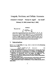
The first step of the computation is to mark all the points on the horizontal axis that correspond to the image of N by f , g and h. Given the recursive definitions of the functions, the automaton will successively mark f (1), g(1), h(1), f (2) etc. The general idea is to mark, after f (k) is constructed, all the points of the form f (k)±g(i)±g(j), f (k)±h(i)±h(j), g(i)±f (j)±f (k) and h(i)±f (j)±f (k) for all i, j < k, and symmetrically after marking g(k) or h(k). If we inductively assume that all the necessary markings have been done, then after marking f (k + 1) and all the corresponding points, a signal can move to the right from g(k) until it reaches the first cell that is not “forbidden” by the definition of g and mark it as being g(k + 1). Also, from the start of the construction, the horizontal axis (y = 0), the vertical axis (x = 0) and the “diagonal axis” (x = y) will be marked by signals going at maximum speed. We will only focus on the construction of the functions on the positive half axes, but the symmetric construction will be made on the negative half axes. Addition and Substraction on the Axes. Let us consider two integers a and b such that 0 < a ≤ b. We assume that both cells (a, 0) and (b, 0) have been marked on the axis at times τ (a) and τ (b) respectively. Then, using constructions as illustrated in figures 1 and 2, it is possible to mark the points (a + b, 0) and (b − a, 0) at times τ (a + b) = max(τ (a) + a + b, τ (b) + 2a) and τ (a − b) = max(τ (a) + b, τ (b) + b) .

(3)

a

b

c (a + b) (a + c) (b + c)

Fig. 1. Additions on a 2DCA

3.2

(c − b) (b − a) a (c − a)

b

c

Fig. 2. Substractions on a 2DCA

Computing the Functions on the X-Axis

In the following section, we will identify the x-axis of Z2 with Z. In other words, we will refer to the cell (n, 0) simply as n. To construct the sets f (N), g(N) and h(N) we will use many different states. Let’s assume that at time τ (n) all the following cell sets are marked on the x-axis (some cells might be in several sets in which case it is marked with a “combination” of states): F = {f (k), k ≤ n}, 2F = {f (k) ± f (k 0 )|k, k 0 ≤ n} = F ± F and F = (±F ± 2G ∪ ±F ± 2H) ∩ N . and the corresponding sets after permutation of f , g and h. Also, we assume that f (n), g(n) and h(n) are in particular states that indicate they are the greatest known points of f (N), g(N) and h(N) and that every point marked on the x-axis (as being part of any of the previous sets) has sent signals diagonally to his right and his left in order to be able to perform additions and substractions as illustrated in the previous paragraph. From here, constructing f (n + 1) is simply a matter of moving a signal from f (n) to the right until it reaches a cell that is not marked as being in F . f (n) “forgets” that it is the last value of F when the signal starts searching for f (n+1) and when f (n + 1) is marked, it “knows” that it is the last known value of F . f (n+1) is also marked as being part of the sets F , 2F , F , G and H. New diagonal signals are sent to the right and the left, that will interact with the existing ones (sent by previously marked points) to mark the cells of the following sets: f (n + 1) ± F ⊆ 2F, 2f (n + 1) ∈ 2F, ±f (n + 1) ± 2G and ±f (n + 1) ± 2H ⊆ F . and then the points in 2F + G ⊆ G and 2F + H ⊆ H since we have changed 2F . In order for the point g(n + 1) to be marked by the same method without error, we have to make sure that the set G has been completely marked. It is easy to see that the last point of this set to be constructed will be 2f (n + 1) + 2g(n).

Using the inequations from (3), we see that it’ll be constructed at most at time 

   τ (f (n + 1)) + 2f (n + 1) + 2 f (n + 1) + 2g(n) = τ (f (n + 1)) + 4(f (n + 1) + g(n)) . where τ (f (n + 1)) is the time when (f (n + 1), 0) is marked as being in F . Therefore, we have to wait 4f (n + 1) + 4g(n) generations before we start looking for g(n + 1). To do so, the cell f (n + 1) will send two signals as soon as it is marked. The first one will move to the left at speed 1/4 while the second one will move to the right at speed 1. Their evolution will only be affected by the cells f (n + 1), g(n) and the origin (0, 0). We are in one of these two possibilities (both cases are illustrated by figures 3 and 4): – 0 < g(n) < f (n + 1), in this case the right signal won’t encounter any important cell and thus will continue to the right forever. On the other hand, the left signal will reach g(n) and remember it (by changing its state), and continue to the origin still at speed 1/4. After reaching the origin, it will turn around and return to g(n) at speed 1/4. When the right signal arrives at g(n) for the second time, it has travelled during 4f (n + 1) + 4g(n) generations. – 0 < f (n + 1) < g(n), in this case, the left signal will go directly to the origin without ever seeing g(n) and will disappear. The right signal however will reach g(n), turn around and go back to f (n + 1) at speed 1, then continue to the origin at speed 1/4 where it turns around and goes to f (n + 1) for the second time at speed 1/4, and finally goes to g(n) at speed 1/2. When it reaches g(n) for the second time, the right signal has travelled during 4f (n + 1) + 4g(n) generations.

g(n)

0 1/4

1

f (n + 1)

0

f (n + 1) 1/4

1/4 ∞

1/4

1

1/4

1/2

1/4

Fig. 3. 0 < g(n) < f (n + 1)

g(n) 1

Fig. 4. 0 < f (n + 1) < g(n)

In both cases, we see that one of the signals reaches g(n) exactly when the last point of G is constructed on the axis, and so g(n) can send a signal to the right to mark g(n + 1). After marking g(n + 1), two signals are sent to wait exactly 4g(n + 1) + 4h(n) generations while the set H is being updated. Then h(n + 1) is constructed, and after waiting long enough, a signal reaches f (n + 1) when F is up to date. At this point we are in the same conditions that the ones we assumed to start constructing f (n + 1) and so the inductive construction of f (N), g(N) and h(N) can continue.

We have the following inequalities: τ (g(n + 1)) ≥ τ (f (n + 1)) + 4f (n + 1) + 4g(n) τ (h(n + 1)) ≥ τ (g(n + 1)) + 4g(n + 1) + 4h(n)) τ (f (n + 2)) ≥ τ (h(n + 1)) + 4h(n + 1) + 4f (n + 1))

(4)

Polynomial Time Bounds. We will now give a rough upper bound of the time needed to construct the functions f , g and h on the x-axis. We assume that τ (f (0)) = τ (g(0)) = τ (h(0)) = 0 since the state of the origin is given in the initial configuration. After marking f (n + 1), we wait exactly 4f (n + 1) + 4g(n) generations before the signal starts propagating to the right from g(n) and g(n+ 1) − g(n) before it reaches its destination. Therefore we have, using the inequalities from (2), for all n ∈ N τ (g(n + 1)) = τ (f (n + 1)) + O(n3 ) And using the corresponding result on f and h, for all n ∈ N τ (g(n + 1)) = τ (g(n)) + O(n3 ) =

n X

O(k 3 ) = O(n4 )

(5)

k=0

We have the same polynomial bound on τ (f (n)) and τ (h(n)). Construction on the Other Axes. When the cell (g(n), 0) is marked as being part of G, a signal is sent in the direction (−1, 1) and it reaches the y-axis on (0, g(n)) after g(n) generations and marks it. Similarly, when h(n) is marked, a signal is sent in the direction (0, 1) that reaches the diagonal axis (x = y) on (h(n), h(n)) after h(n) generations. 3.3

Computation of the Rest of t(Z3 )

We will consider here the norm 1 on Z3 (||(a, b, c)|| = |a| + |b| + |c|). The sphere of radius k for this norm will be denoted as Sk . Let p = (x, y, z) ∈ Z3 , with ||p|| = k. We will say that p0 = (x0 , y 0 , z 0 ) is a superior neighbor of p (and that p is an inferior neighbor of p0 ) if p0 ∈ Sk+1 and ||p0 − p|| = 1. In Z2 we will say that t(p0 ) is a superior t-neighbor of t(p). The number and the position (relative) of the superior neighbors of p only depend on the signs of p’s coordinates. Also, every point that is not on one of the axes (in Z3 ) has at least two inferior neighbors (one for each non-zero coordinate). Inductive Construction. We will see here how it is possible to inductively construct the images by t of all the spheres Sk . Since it is not possible to give each cell in t(Z3 ) the number of the sphere it is in (this would require an infinite number of states) we will consider two cell sets S+0 and S+1 that will represent, for each step k of the induction, the current sphere (Sk ) and the next one (Sk+1 ). During step k we will construct Sk+2 . For k0 ∈ N, let’s assume we are in a configuration such that:

– For all p ∈ Sk0 , the cell t(p) is in S+0 and knows the sign of each of p’s coordinates (and so knows the direction in which each of its superior tneighbors is). Reciprocally, every cell in S+0 is the image of a point of Sk0 . – For all p ∈ Sk0 +1 , the cell t(p) is in S+1 and knows the sign of each of p’s coordinates (it knows where its inferior t-neighbors are). Also, every cell in S+1 is the image of a point of Sk0 +1 . Such a situtation is illustrated on the figure 5 for k0 = 1.

Fig. 6. The signals s1 (black) and s2 (dashed grey) during step 1 Fig. 5. The spheres S1 (black squares) and S2 (grey circles)

In this situation, a signal s0 is sent from the origin (we will explain later what causes this signal to appear) in all directions and spreads at maximum speed forming a square around the origin. When a cell in S+0 receives this signal, it sends a signal s1 to each of its superior t-neighbors and, after doing so, is no longer in S+0 . When a cell in S+1 receives a signal s1 , the signal disappears and the cell sends a signal s2 to each of its superior t-neighbors except the one that is the direction of the received signal (this is illustrated in figure 6 for the upper right quarter of Z2 ). The upper t-neighbors of these cells are not yet constructed but the cells know in which direction they are because they know the coordinates of their corresponding point in Z3 . When a cell in S+1 has received a signal s1 from all its inferior t-neighbors it becomes a cell of S+0 and is no longer in S+1 . Since the signal s0 spreads at maximum speed we are sure that it cannot interact with these cells (but it will during the next step of course). When two s2 signals meet on a cell, they both disappear and the cell is marked as being in S+1 (again, this cell won’t do anything before the next step since it won’t receive any s1 signal). Also, the direction of the s2 signals that arrive to a cell indicate the position of its inferior t-neighbors so when all signals

have arrived, the cell knows where all its superior t-neighbors are. Note that a given cell can (and most of the time will) receive more than one couple of s2 signals. Each time, the signals disappear, and the cell gets more information from the inferior t-neighbors. This construction marks all cells in t(Sk0 +2 ) that have at least two inferior t-neighbors. Only the ones on the axes are left, and they are constructed independently as explained earlier. Correctness of the Construction. The correctness of this construction is based on two observations. First, there cannot be any conflict between the s1 and s2 signals because between a cell of t(Z3 ) and one of its superior t-neighbors there is no other cell of t(Z3 ). Second, if we consider a point p ∈ Sk0 +2 having at least two inferior neighbors p1 and p2 , then these two points share a common inferior t-neighbor p0 because p1 and p2 can be obtained from p by reducing one of the coordinates (a different one for each), and so p0 can be obtained by reducing both coordinates from p. Moreover, the basic properties of t ensure that the points t(p), t(p1 ), t(p2 ) and t(p0 ) form a parallelogram. So the paths p0 → p1 → p and p0 → p2 → p have same length and so the two s2 signals will meet on p (see figure 6). Every cell in t(Sk0 +1 ) will therefore receive a couple of coinciding s2 signals for each couple of its inferior neighbors, and so will be able to deduce the signs of all coordinates of the point in Z3 it is the image of. Synchronisation. The previously explained construction relies on a signal s0 that will initiate it. This signal must appear after all points of Sk0 and Sk0 +1 are marked as being in S+0 and S+1 respectively. Since the construction is inductive, it is obvious that Sk0 +1 will be marked after Sk0 . Therefore, it is sufficient to ensure that the signal s0 (corresponding to step k0 ) appears after Sk0 +1 is fully marked. To do so, let’s create a signal from (h(k0 + 1), 0) when the cell is marked as being in h(N) (at time τ (h(n))) that will move left at speed 1, and will trigger the s0 signal when reaching the origin. Let’s prove the construction by induction. For some k0 ∈ N, let’s assume that all points of Sk0 +1 are marked at time τs (k0 ) = τ (h(k0 + 1)) + h(k0 + 1) (when the signal s0 from step k0 appears). Then s0 reaches all points in Sk0 by time at most τs (k0 ) + max(f (k0 ), g(k0 )) + h(k0 ) and the propagation of signals s1 and s2 lasts at most 2 max(f (k0 + 1) − f (k0 ), g(k0 + 1) − g(k0 ), h(k0 + 1) − h(k0 )) In the end, all points of Sk0 +1 that are marked by these signals are marked at time at most    f (k0 + 1) − f (k0 ) f (k0 ) + h(k0 ) + 2 max g(k0 + 1) − g(k0 ) τ (h(k0 + 1)) + h(k0 + 1) + max g(k0 ) + h(k0 )  h(k0 + 1) − h(k0 )

It is easy to see that this time is lower than τ (h(k0 + 1)) + h(k0 + 1) + 2f (k0 + 1) + 2g(k0 + 1) + 2h(k0 + 1) And if we use the inequalities from (4) we get τs (k0 + 1) = t(h(k0 + 2)) + h(k0 + 2) ≥ τ (h(k0 + 1)) + 4h(k0 + 1) + 4f (k0 + 2) + 4g(k0 + 2) + h(k0 + 2) ≥ τ (h(k0 + 1)) + h(k0 + 1) + 2f (k0 + 1) + 2g(k0 + 1) + 2h(k0 + 1) Also, the only points in t(Sk0 +2 ) that are not constructed by the signals s2 are the ones on the axes. There are six of them: ±(f (k0 + 2), 0), ±(0, g(k0 + 2)) and ±(h(k0 + 2), h(k0 + 2)), and they are marked at times τ (f (k0 + 2)), τ (g(k0 + 2)) + g(k0 + 2) and τ (h(k0 + 2)) + h(k0 + 2) respectively, all lower than or equal to τs (k0 + 1). Therefore, when the signal s0 from step k0 + 1 is triggered all points of Sk0 +1 and Sk0 +2 are marked and the construction can be done correctly. 3.4

End of the Construction

The last thing to do now is to “activate” the cells in t(Z3 ) when all of their t-neighbors have been constructed (we will need this information later when simulating A3 ). To do so, since every point of t(Z3 ) knows the direction where all its inferior t-neighbors are when it is constructed, it will send a special “activation” signal to them as soon as it is marked. When a given cell has received an “activation” signal from all its superior t-neighbors it goes into a new “activated” state. We have therefore seen in this section how it is possible to construct, using a 2DCA working on Moore’s neighborhood starting on the configuration where all cells are in a quiescent state except the origin, the image of Z3 by t. This construction is done in polynomial time, meaning that the image of the sphere Sk , which is of radius O(k 3 ) as seen in (2) is constructed in time O(k 4 ) (according to (5) and the arguments of induction). This ends the proof of theorem 2.

4

Description of A2

The final 2DCA A2 is a superposition of two 2DCA working in parallel. The lower layer is the one that will mark t(Z3 ) during the simulation as explained previously. We will represent the evolution of this construction by colors. A cell that has been marked as part of t(Z3 ) but has not yet been activated (its tneighbors are still being constructed) will be represented as grey. A cell marked and activated will be either black or red (we will see later why we need two colors) and a cell that hasn’t been marked is white. We will say that a cell is colored if it is either grey, black or red (as opposed to white). The upper layer is the one that will really do the simulation.

Colored cells all correspond to a cell of A3 . Their state will be a product of information. What we will call their central state is the state of their corresponding cell that they are currently simulating. A red cell will send signals containing its central state in the directions of its t-neighbors. The next generation, it becomes black so that the central state is sent only once. These signals are transmitted by white cells. When a black cell receives one of these signals, the signal disappears and the cell memorizes the state of the corresponding tneighbor (which neighbor depends on the direction the signal came from). When it knows all the central states of its t-neighbors, the black cell applies the transition function of A3 , changes its central state and becomes red (to transmit the new central state)... 3

Given a configuration C3 ∈ Q3Z , the initial configuration of A2 is as follows. The lower layer is initialized on the origin only (all other cells are in the blank state) to construct t(Z3 ) as we have seen. If C3 is finite (only a finite number of cells are not in the blank state q0 ), for all c ∈ Z3 such that C3 (c) 6= q0 , t(c) receives C3 (c) as its central state. All other cells are left blank, so the initial configuration of A2 is finite too. If C3 is infinite, all cells in t(Z3 ) receive the state of their preimage. As the construction of t(Z3 ) by the lower layer goes on, cells become grey (marked but not activated) and then they are activated and become red. A new red cell either has a central state given initially, or it is initialized as q0 when the cell is activated. Note that grey cells gather informations about their t-neighbors like black cells do but don’t send their central state because some of their t-neighbors aren’t marked yet and the signals might be lost. It is important to see that the simulation of A3 by A2 is therefore asynchronous because the colored cells apply the transition function of A3 at different times. This means that the number of A3 generations computed by the colored cells isn’t the same for all. However, there is a dependency between a cell and its t-neighbors that ensures that, at a given time τ , each colored cell t(c) has computed at most one generation more than any of its t-neighbors. This gives a sort of partial-synchronicity and proves that a black or grey cell can never receive more than two consecutive signals from any of its t-neighbors before it can process them, and so each cell can have only a finite memory. This automaton simulates A3 in the sense that for a given configuration C3 , for any cell c ∈ Z3 , the sequence of states of c in the evolution of A3 starting on C3 is exactly the sequence of central states of t(c) restricted to the times when t(c) is red. The time needed for a given cell t(c) to compute k generations of its corresponding cell c is at most the time needed to activate all the image by t of the sphere of radius k centered on c, plus the radius of the image of this sphere (it’s the time needed for the furthest information to reach t(c)). We have seen that these spheres grow polynomially, and that they are constructed in polynomial time so for every cell c ∈ Z3 there exists a polynomial Pc ∈ Z[X] of degree at most 4 such that t(c) has computed k generations of c in time at most Pc (k). Note that the polynomial depends on c but considering the relative sizes of the

spheres of radius k in Z3 and Z2 it is easy to prove that we cannot simulate k generations of A3 on Z2 in a time bounded by a global polynomial (it is in fact impossible to bound it by any function).

5

Conclusion

What we have done here can easily be done to simulate any n-dimensional CA on a 2DCA. However doing such a construction to simulate a 2DCA with a 1DCA doesn’t work (mainly because we cannot embed as we did the 2D neighborhood in a 1D neighborhood and use a similar construction without important conflicts). Many things can now be studied about this simulation. For example, the f , g and h functions used here are bounded by polynomials of degree 3. Considering the size of the spheres, we see that it is not possible to have polynomials of degree lower than 3/2 but where exactly is the real lower bound of the simulation? Also the irregularity of the functions that we use here make them hard to compute with a 2DCA, but having a better understanding of their growth (a good lower bound) or finding simpler functions (still bounded polynomially) could highly improve the construction in terms of time and number of necessary states. The automaton constructs a representation of Z3 in Z2 . It would be interesting to study how usual 3-dimensional objects are represented, and if natural 3-dimensional cellular automata configurations can be identified easily after projection. We have seen here how to encode finite configurations of A3 as finite configurations of A2 . Periodic A3 configurations can also be simulated by a 2DCA using a method similar to the one described if we encode them as finite configurations of A2 using specific state markers for the borderline and sending the signals from one border to the other (as on a torus).

References 1. Frisch, U., d’Humi`eres, D., Hasslacher, B., Lallemand, P., Pomeau, Y., Rivet, J.P.: Lattice gas hydrodynamics in two and three dimension. Complex Systems 1 (1987) 649–707 Reprinted in Lattice Gas Methods for Partial Differential Equations, ed. G. Doolen, p.77, Addison-Wesley, 1990. 2. R´ oka, Z.: Simulations between cellular automata on Cayley graphs. Theoretical Computer Science 225 (1999) 81–111 3. Martin, B.: A geometrical hierarchy on graphs via cellular automata. Fundamenta Informaticae 52 (2002) 157–181 4. Cole, S.N.: Real-time computation by n-dimensional iterative arrays of finite-state machines. IEEE Transactions on Computers C-18 (1969) 349–365