Scanning Electron Microscopy - MBG

JEOL 5000 Neoscope

Light Microscope Resolution - The best resolution of the light microscope is 0.2 µm or 200 nm. Magnification - to the magnification, in addition to the resolution. The highest useful magnification of an objective lens in the light microscope is 100 times. When you look through the eyepiece this often adds another 10 times magnification. Thus, the highest magnification of the light microscope is 1000 times. SEM Resolution -The resolution of our SEM (Neoscope) is 3 to 6 nm. That's almost 100 times better than the light microscope. This is why we can see so much more detail with electron microscopes than light microscopes. Magnification - The highest magnification of our scanning electron microscope is 20,000 times! That's 20 times more than the light microscope. They go up to 1,000,000X.

JEOL SEM from 2008

Exfoliated graphite with nanoparticles, 1,000,000X

Fullerene (Buckyball) colloids, 1,000,000X

Scanning Electron Microscopy - MBG

Neoscope SEM Gun and Vacuum Column

Neoscope Sample Chamber, X-Y Controls

Volumes within the specimen where signals are generated

Detecting Secondary Electrons

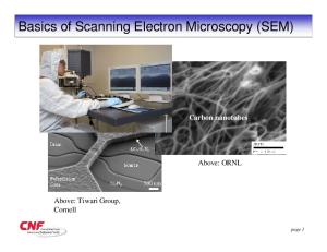
The SEM provides two outstanding improvements over the optical microscope: it extends the resolution limits and improves the depth-of-focus resolution more dramatically (by a factor of ~300). The SEM is also capable of examining objects at a large range of magnifications. This feature is useful in forensic studies as well as other fields because the electron image complements the information available from the optical image.

History of SEM 1920s – particle wave theory 1931 – first TEM built, Ernst Ruska and Max Knoll 1935 – SEM developed by Knoll 1938 – first SEM built – Von Ardenne 1956 – electromagnetic lens improved 1960 – improved SEM detector 1965 – first commercial SEMs, Cambridge 1982 – first CCD devices used with SEM

History of SEM

1931 – first TEM Ernst Ruska Max Knoll

used two magnetic lenses, and three years later a third lens was added, demonstrating a resolution of 100 nm, twice as good as that of the light microscope

TEM Microscopes Model built by Ruska in 1933

Current model

Sauromatum guttatum Araeceae, TEM Parenchyma cell

Bacillus anthracis – Anthrax, SEM

TEM – Golgi apparatus

SEM – stem cell

Max Knoll’s Electron Beam Scanner

Manfred von Ardenne – SEM design

Prof. Oatley’s Group SEMs – 1950’s and 1960’s

Photograph device added

Magnetic focus added

1967 - Stereoscan Mark VI – Cambridge Instruments An early commercial SEM

JEOL – first commercial SEM, 1966

The JSM (now known as the JSM-1 was JEOL's first commercially produced Scanning Electron Microscope. The JSM -1 was made commercially available in 1966. Among its advanced features was a Eucentric Stage. Resolution: 250Å (at 25kV) Magnification: 100 - 30,000 Scan area: 1x1 mm (at 25kV)

Vacuum System A vacuum is required when using an electron beam because electrons will quickly disperse or scatter due to collisions with other molecules.

Electron beam generation system. This system is found at the top of the microscope column, and generates the "illuminating" beam of electrons known as the primary (1o) electron beam.

Electron beam manipulation system. This system consists of electromagnetic lenses and coils located in the microscope column and control the size, shape, and position of the electron beam on the specimen surface.

Condenser lens converges the electron beam generated from the electron gun to a fine electron beam

Scanning coils generate the “raster” beam that scans back and forth on the specimen. The electron beam is scanned across the specimen by scan coils while a detector measures the radiation emitted from the specimen.

Magnetic Lens A magnetic lens consists of a coil of copper wires inside the iron pole pieces. A current through the coils creates a magnetic field (symbolized by red lines) in the bore of the pole pieces. The rotationally symmetric magnetic field is inhomogeneous in such a way that it is weak in the center of the gap and becomes stronger close to the bore. Electrons close to the center are less strongly deflected than those passing the lens far from the axis. The overall effect is that a beam of parallel electrons is focused into a spot (so-called cross-over).

Lens Aberrations - Astigmatism: Strength of lens is asymmetrical; it is stronger in one plane than another. Caused by machining errors, nonhomogeneous polepiece iron, asymmetrical windings, dirty apertures. Results in out-of-focus “stretched” image. Corrected with stigmator coils.

Beam specimen interaction system.

This system involves the interaction of the electron beam with the specimen and the types of signals that can be detected.

Detection system. This system can consist of several different detectors, each sensitive to different energy / particle emissions that occur on the sample.

Signal processing system. This system is an electronic system that processes the signal generated by the detection system and allows additional electronic manipulation of the image. Signal manipulation begins with the amplifier in the detector and ends with the image on the viewing screen. All controls associated with the changing the way the image is viewed in terms of brightness and contrast is considered part of the signal manipulation system

Display and recording system. This system allows visualization of an electronic signal using a cathode ray tube and permits recording of the results using photographic or magnetic media. Factors that determine the quality of a micrograph Brightness – value of pixels in image Contrast – difference between highest and lowest pixel Resolution - size of the beam spot, working distance, aperture size, beam bias current, voltage, and how cylindrical the beam is Magnification - function of area scanned and viewing size Depth of field - region of acceptable sharpness Noise - any level of brightness observed in a micrograph, white or black, that is not a result of the planned interaction of the beam with the specimen Composition - all the above characters plus the way the subject is framed

Sample Preparation Size -Maximum size approximately 1 cm in diameter Clean – free of oil, resins, loose parts, debris, dust Dry - completely dehydrated prior to being placed in the microscope chamber Conductive or non-conductive Biologicals Powders, loose parts Plane, angularity, shape, parts sticking out

SEM Stubs

Carbon Paint

Carbon Tape

Stub Adhesives Copper Tape

Silver Paint

Pelco Adhesive Pads

Scanning Electron Microscopy - MBG

Sharon Carter – 2012 REU

Neoscope SEM Control Panel

Rose Petal – sample prep CPD

Fixed and Air-Dried

Denton Desk V Sputter Coater

Sputter Coating

Critical Point

The phase diagram shows the pressure to temperature ranges where solid, liquid and vapor exist. The boundaries between the phases meet at a point on the graph called the triple point. Along the boundary between the liquid and vapor phases it is possible to choose a particular temperature and corresponding pressure, where liquid and vapor can co-exist and hence have the same density. This is the critical temperature and pressure.

EMS 850 - features built-in chamber cooling and heating,

Specimen holder

12 Chambers

12 Porous pots

Raised stomatal pore

Bamboo Stem

CPD – starch amyloplasts

CPD - glands

Principal features of a light microscope, a transmission electron microscope (TEM), and a scanning electron microscope (SEM), drawn to emphasize the similarities of overall design. The TEM and SEM require that the specimen be placed in a high-vacuum environment.

Celastrus orbiculatus

Opuntia humifusus

Rhododendron sp.

Mendoza – Hydrocotyle fruits

Nallarett Davila – Rubiaceae Parque Virua

Colleters

Shaw Institute for Field Studies - High School Students

BrieAnna Langlie – carbonized potato, 3,000 bp

Jinshun Zhong – Lamium apices

Katie Parks Monarda

Peris Kamau – Pteris spores from Africa

Rachel Hillabrand – Lythraceae Seed Walls

End