Scanning Electron Microscope (SEM)

High Temperature Materials KGP003 Div. of Process Metallurgy Spring 2006

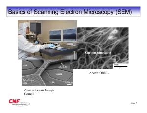
SCANNING ELECTRON MICROSCOPY (SEM): In the scanning electron microscope (SEM) a very fine 'probe' of electrons with energies up to 40 keV is focused at the surface of the specimen in the microscope and scanned across it in a 'raster' or pattern of parallel lines. A number of phenomena occur at the surface under electron impact: most important for scanning microscopy are the emission of secondary electrons with energies of a few tens eV and re-emission or reflection of the high-energy backscattered electrons from the primary beam. The intensity of emission of both secondary and backscattered electrons is very sensitive to the angle at which the electron beam strikes the surface, i.e. to topographical features on the specimen. The emitted electron current is collected and amplified; variations in the resulting signal strength as electron probe is scanned across the specimen are used to vary the brightness of the trace of a cathode ray tube being scanned in synchronism with the probe. There is thus a direct positional correspondence between the electron beam scanning across the specimen and the fluorescent image on the cathode ray tube. The magnification produced by scanning microscope is the ratio between the dimensions of the final image display and the field scanned on the specimen. Usually magnification range of SEM is between 10 to 200 000 X. and the resolution (resolving power) is between 4 to 10 nm (40 - 100 Angstroms) . There are many different types of SEM designed for specific purposes ranging from routine morphological studies, to high-speed compositional analyses or to the study of environment sensitive materials. Our laboratory has a combination SEM and EDS, which in combination, provide a powerful analytical approach for many research or quality control applications. Here is example of using SEM in the material research.

The left image shows a Nimonic 115 heat and corrosion resistant wrought nickel alloy that has not been exposed to excessive overheating. There is no evidence of significant growth of

-2-

gamma prime precipitates. By using the backscattered electrons, two phases differing only slightly in composition, can be distinguished. The right image shows the effect of overheating. The material was exposed to a temperature of 1200 C. The grain boundary has been effected, two phases have disappeared and the structure of the edges has changed. The dark lobes correspond to an aluminum rich phase. A

typical triangular precipitate at the end of the "crack" can also be seen. It is composed of titanium with a few percent of nitrogen. ENERGY DISPERSIVE SPECTROSCOPY (EDS): Chemical analysis (microanalysis) in the scanning electron microscope (SEM) is performed by measuring the energy or wavelength and intensity distribution of X-ray signal generated by a focused electron beam on the specimen. With the attachment of the energy dispersive spectrometer (EDS) or wavelength dispersive spectrometers (WDS), the precise elemental composition of materials can be obtained with high spatial resolution. When we work with bulk specimens in the SEM very precise accurate chemical analyses (relative error 1-2%) can be obtained from larger areas of the solid (0.5-3 micrometer diameter) using an EDS or WDS. Bellow is an example of EDS spectrum collected in the SEM with EDS. The spectrum shows presence of Al, Si, Ca, Mn and Fe in the steel slag phase.

-3-

THE PRINCIPLES BEHIND SEM:

Electron gun

Condenser lenses

Vacuum pump

Aperture Scan coils Objective lens

Detector

Vacuum pump

SEM sample

Electron Beam In a SEM the electron beam energy and current are variables. The voltage is variable from about 1 - 60keV and the current from 1e-7 to 1e-12 A. These are rough guidelines - the exact ranges available depend on the instrument type and manufacturer. Condenser lenses

These magnetic lenses focus an image of the electron gun onto the aperture, in order to spatially filter the electron beam. Aperture Controls the spread of electrons in the column by de-selecting off-axis electrons. Vacuum pumps The specimen chamber and the column must both be evacuated, in order to prevent scattering of the beam electrons by air molecules. Electron gun Several different types of electron gun are used in SEMs, the most primitive being a simple tungsten "hairpin" filament. The filament is heated by passing a current through it, and electrons are then emitted via the process of thermionic emission. The effective size of this

-4-

electron source (and hence the final electron spot size) can be reduced by instead using a single crystal of lanthanum hexaboride (LaB6). Still finer resolution can be achieved using an almost atomically sharp single crystal tungsten tip, which allows electrons to be emitted by a field emission process. Scan coils These coils deflect the beam in order to scan the electron spot in a raster pattern across the sample. Objective lens This magnetic lens focuses the electron beam onto the sample. Detector At each beam position, some quantity or characteristic of the sample must be measured, so that an image can be built up. The most commonly measured quantity is the rate of secondary electrons emitted from the sample, and this is detected by using a scintillator in conjunction with a photomultiplier. SEM sample Conducting samples provide a path to earth for the beam electrons, and therefore require no special preparation. Insulating materials, however, require a thin coating of a conductor (often carbon or gold) in order to prevent charging. DIFFERENT SEM MODES: Primary electron imaging When an electron from the beam encounters a nucleus in the sample, the resultant Coulombic attraction results in the deflection of the electron's path, known as Rutherford elastic scattering. A few of these electrons will be completely backscattered, re-emerging from the incident surface of the sample. Since the scattering angle is strongly dependent on the atomic number of the nucleus involved, the primary electrons arriving at a given detector position can be used to yield images containing both topological and compositional information. Secondary electron imaging The high-energy incident electrons can also interact with the loosely bound conduction band electrons in the sample. The amount of energy given to these secondary electrons as a result of the interactions is small, and so they have a very limited range in the sample (a few nm). Because of this, only those secondary electrons that are produced within a very short distance of the surface are able to escape from the sample. This means that this detection mode boasts high-resolution topographical images, making this, the most widely used of the SEM modes.

-5-

Energy-Dispersive analysis of X-rays (EDX) Another possible way in which a beam electron can interact with an atom is by the ionization of an inner shell electron. The resultant vacancy is filled by an outer electron, which can release it's energy either via an Auger electron or (more importantly here) by emitting an Xray. This produces characteristic lines in the X-ray spectrum corresponding to the electronic transitions involved. Since these lines are specific to a given element, the composition of the material can be deduced. This can be used to provide quantitative information about the elements present at a given point on the sample, or alternatively it is possible to map the abundance of a particular element as a function of position. Linescan (qualitative) The electron probe traverses along the line on the surface of stationary sample. Line scanning produces graphs of elemental distributions across boundaries and through phases in sample. This method is very illustrative for showing concentration gradients e.g. at grain or phase boundaries. Linescan (quantitative) The specimen is traversed along a predetermined line at steady rate with the help of the stage stepping motors. After every step the specimen stops and quantitative element analysis is performed. The number and the length of steps on the line are controllable. Element map Along with a video image the distribution of predetermined elements is obtained for the observed image area. The video and element images can easily be superimposed into a composite image. This is excellent eg. for observing adjoining phases of different composition, microchemical composition of inclusions in steel, and distribution of impurities on the sample surface.

-6-

EXAMPLES:

SEM-X-ray mapping

This Micrograph shows a secondary electron image of the cadmium telluride surface of a polycrystalline CdS/CdTe cell.

Iron oxide

Cancer Cells

-7-

X-RAY DIFFRACTION (XRD)

High Temperature Materials KGP003 Div. of Process Metallurgy Spring 2006

-8-

Background: X-rays are electromagnetic radiation of wavelength about 1 Å (1x10-9 m), which is about the same size as an atom. They occur in that portion of the electromagnetic spectrum between gamma rays and the ultraviolet. The discovery of X-rays in 1895 enabled scientists to probe crystalline structure at the atomic level. X-ray diffraction has been in use in two main areas, for the fingerprint characterization of crystalline materials and the determination of their structure. Each crystalline solid has its unique characteristic X-ray pattern that may be used as a "fingerprint" for its identification. Once the material has been identified, X-ray crystallography may be used to determine its structure, i.e. how the atoms pack together in the crystalline state and what the interatomic distance and angle are etc. X-ray diffraction is one of the most important characterization tools used in solid-state chemistry and materials science. The XRD technique requires only a small amount of material and is non-destructive so that further analysis can be completed on the same material afterwards.

The workings of a modern x-ray diffractometer are quite complex but the general layout and geometry is given in Figure 1. The basic components of an XRD diffractometer are the x-ray source, the sample specimen and an x-ray detector.

Fig. 1 Arrangement and geometry of an x-ray diffractometer The X-ray radiation most commonly used is that emitted by copper, whose characteristic wavelength for K radiation is =1.5418Å. When the incident beam strikes a powder sample, diffraction occurs in every possible orientation of 2θ. The diffracted beam may be detected by using a moveable detector such as a Geiger counter, which is connected to a chart recorder. In normal use, the counter is set to scan over a range of 2θ values at a constant angular velocity.

-9-

Routinely, a 2θ range of 5 to 70 degrees is sufficient to cover the most useful part of the powder pattern. The scanning speed of the counter is usually 1-2 degrees/min and therefore, about 30 minutes to 1 hour is needed to obtain a trace. Theory: A crystal system can be thought of as a structure built from unit cells that, when stacked, fill three-dimensional space. There are seven discrete unit cell shapes in three-dimensional space. These seven unit cell shapes are known as the seven crystal systems: triclinic, monoclinic, orthorhombic, tetragonal, hexagonal, rhombohedral, cubic. Each point in a unit cell is an atom within the crystal structure. Hence, the physical aspects of crystal structure on an atomic level are possible to investigate using XRD. The concept of XRD is based on Bragg’s law, λ=2dsinθ. Where λ is wavelength, d is the interplanar distance between atoms in the crystal and θ is the incident and reflection angle of x-rays.

Fig. 2 Reflection of x-rays from two planes of atoms in a solid Figure 2 illustrates the path difference between two x-rays reflecting from two planes of atoms in a crystal: 2λ = 2dsinθ

For constructive interference (destructive interference cancels the reflection) between these xrays, the path difference must be an integral number of wavelengths:

This leads to the Bragg equation: nλ= 2dsinθ

- 10 -

Figure 3 shows the x-ray diffraction pattern from a single crystal of layered clay. Strong intensities can be seen for a number of values of n, i.e. different atomic planes; from each of these lines we can calculate the value of d, the interplanar spacing between the atoms in the crystal.

Fig. 3 X-ray diffraction pattern from layered structure vermiculite clay EXAMPLE: Unit Cell Size from Diffraction Data

The diffraction pattern of copper metal was measured with x-ray radiation of wavelength of 1.54 Å. The first order Bragg diffraction peak was found at an angle 2θ of 69.32 degrees. Calculate the spacing between the diffracting planes in the copper metal. The Bragg equation is: nλ = 2dsinθ We can rearrange this equation for the unknown spacing d: d = nλ/2sinθ θ is 34.66 degrees, n =1, and wavelength = 1.54 Å, and therefore d= 1 x 1.54/(2 x 0.5687) = 1.354 Å Practical Application:

What criteria should a powder sample have to be suitable for XRD? •

Suitable grain size The size should be between 70 μm (high symmetry) of 50 μm (lower symmetry) to about 0.5 μm. Overly small grain sizes give peak broadening. Overly large grain sizes give preferred orientation and “spotty” peaks. Use a mill, but not for too long or you will create amorphous material! (noncrystalline).

•

Randomly oriented crystals

- 11 -

The sample loading into the specimen holder is important. Do not work with the sample more than necessary, otherwise preferred orientation may occur and alter the relative intensity of the resulting peaks. •

Flat, smooth and aligned

Theoretically a curved sample would be optimal (better focusing) but most specimen holders have a flat design for ease of loading. The sample must be aligned at the correct height, otherwise a height error will shift the 2θ scale. •

Suitable sample area

The length of the x-ray beam is about 12 mm on the sample and the width is controlled by slits. We often use variable slits so that the width is 20 mm independent of θ. If the sample size is too small, the intensity will be lowered. •

Suitable sample thickness

The x-rays penetrate a few micrometers into the sample surface, therefore, the sample should be thicker than this. •

Homogenous

If a standard powder is added to the sample, mix them thoroughly in order to maintain a relative homogenous sample. •

Avoid using amorphous sample holders

If you still want to use for instance a glass slide as sample holder, take in to account that the glass can add amorphous pattern to your sample original highly crystalline pattern.

How to identify an unknown sample with XRD? •

Identify the three most intense reflections and determine their d-spacing

•

Search for corresponding d-values in a reference (Hanawalt Search Manual, computer software such as EVA), start with the most intense peak and work in descending order of peak intensity

•

After finding the d-values which correspond the best with d-values from the sample compare the intensities of the sample reflections with the reference reflections

•

Compare d and intensity values for the entire diffractogram, only when full agreement with reference values has been reached is the identification of unknown sample complete.

- 12 -

THERMAL ANALYSIS

DSC /(mW/mg) Ion Current *10-8 /A ↓ exo 1.5

TG /% 100.0 1 ml CO2 pulse

95.0

4

Sample: NaHCO3 amu 44 (CO2)

90.0

2 NaHCO3 -> Na2CO3 + H2O + CO2

1.0

157.7 °C

2

85.0

-36.80 % (theor. 36.90%)

80.0

452.04 J/g

0

0.5

0.25 ml CO2 pulse

75.0 -2 70.0

0.436 mg

65.0

-> 1.34 mg evolved (theor. 1.30 mg)

0

1.745 mg

-4

60.0

-0.5 50

100

150

High Temperature Materials KGP003 Div. of Process Metallurgy Spring 2006 - 13 -

200 Temperature /°C

250

300

Background: Thermal analysis includes a group of methods by which the physical and chemical properties of a substance, a mixture and/or reaction mixtures are determined as a function of temperature or time, while the sample is subjected to a controlled temperature program. The program may involve heating or cooling (dynamic), or holding the temperature constant (isothermal), or any combination of these. TGA stands for Thermo-Gravimetric Analysis. TGA can be used for the determination of decomposition weight loss, combustion analysis, temperature stability, and moisture content and reaction mechanism. TGA monitors weight versus temperature. It can detect changes in weight of 1 ug. This is accomplished with an extremely sensitive balance hanging inside a furnace. A thermocouple mounted just a few millimeters from the sample pan ensures accurate temperature of the sample. There are several events that can be calculated for any run. Thermal Analysis methods: Differential Thermal Analysis (DTA) Differential Scanning Calorimetry (DSC) Thermogravimetry (TG) Simultaneous Thermal Analysis (STA) Thermomechanical Analysis (TMA) Dilatometry (DIL) Dynamic Mechanical Analysis (DMA) Combined (Hyphenated) Techniques (TA - MS, TA - FT-IR, PTA) Thermal Conductivity Testing (TCT) Thermal Diffusivity Measurement (LFA) Refractories Testing (RUL, CIC, MOR) THERMOGRAVIMETRY (TG): This is a technique by which the mass of the sample is monitored as a function of temperature or time, while the sample is subjected to a controlled temperature program. dm/dt DTG DTG Peak Tonset Composition

= = = = =

Dm = mass change rate of mass change/decomposition derivative thermogravimetry characteristic decomposition temperatures ® identification thermal stability moisture content, solvent content, additives, polymer content, filler content , dehydration , decarboxylation, oxidation, decomposition.

The curve of thermogravimetry analysis is build around a furnace where the sample is mechanically connected to an analytical balance. The first thermobalance was developed by

- 14 -

K. Honda in 1915. I t be came widespread from 1950s when the derivated thermogravimetric (DTG) was solved.

Balance, furnace and control/data handling system are the three essential parts of a modern TG instrument. There are three main possibilities to place the sample relative to the balance: a- suspended, b- horizontal, c- top-loading see figure 2.

Figure1 – Schematic of Thermogravimetry system

A

B Figure 2 – Position of the sample in thermobalance

- 15 -

C

DIFFERENTIAL THERMAL ANALYSIS (DTA): DTA is a technique measuring the difference in temperature between a sample and a reference (a thermally inert material) as a function of time or the temperature, when they undergo a temperature scanning in a controlled atmosphere. The DTA method enables any transformation to be detected for all the categories of materials. Applications: Melting and crystallisation behavior, Heat of melting and crystallisation, Heat of reaction, Reaction kinetics, Glass transitions, Oxidative stability, Thermal stability. DIFFERENTIAL SCANNING CALORIMETRY (DSC): DSC is a technique which determines the variation in heat flow released or captured by a sample when it undergoes temperature scanning in a controlled atmosphere. When heating or cooling, any transformation taking place in a material is accompanied by an exchange of heat; DSC enables the temperature of this transformation to be determined and the heat from it to be quantified. Calibration is necessary. 1.

Power compensated DSC

2.

Heat flux DSC

3.

Applications, see DTA

SIMULTANEOUS THERMAL ANALYSIS (STA): This technique combines thermogravimetry with differential thermal analysis or differential scanning calorimetry in one run. - Possible to consider the real sample mass at a given temperature in Cp determination. - No temperature differences between signals of TG and DTA/DSC measurement. Simultaneous Thermal Analysis (STA) is used for the following applications:

Characteristic temperatures

Polymorphism

Identification

Solid-liquid ratio Specific heat capacity

Glass transitions Melting and crystallization behavior

Reaction behavior Heat of reaction

Heat of melting and crystallization Reaction kinetics Oxidative stability

- 16 -

COMBINED (HYPHENATED) TECHNIQUES: With these thermoanalytical methods, for example TG-DTA-MS (ThermogravimetricDifferential Thermal-Mass Spectrometric analysis), the gases evolved from the sample during a thermal analysis experiment are detected/analyzed. APPARATUS (STA 409C) The STA 409C instrument consists of the following main parts (see figure 3): Registration control cabinet, Measuring part, Computer system with printer, Thermostat, Evacuating system (vacuum pump)

TA-controller

measuring part

Computer sustem

printer control cabinet 1 0

thermostat vacuum pump

20 °

Figure 3 – Assembly diagram of STA 409 C/7/E measuring equipment The schematics of STA 409C and STA with QMS are shown in figures 4 and 5 respectively. The balance and furnace are sequentially evacuated and purged with inert gas. Two programs are used with this instrument. One for setting operating conditions, running the STA and data acquisition, another for evaluating the data obtained. In order to avoid buoyancy effect, a TG/DTA correction must be run with empty crucibles and the data obtained will be used as reference when running with a crucible containing sample.

- 17 -

Gas outlet

Furnace

DSC and TG carrier

Sample carrier radiation shield thermostatic control

protective tube vacuum reactive gas protective gas

inductive displacement transducer electromagnetic compensation system

evacuation system

vacuum tight casing

Figure 4 - Scheme of STA-409 C (B).

Figure 5 – Schematic of Skimmer THE QUADRAPOLE MASS SPECTROMETER: The quadrapole mass filter was originally proposed by W. Paul Its basic design is illustrated in figure 6. In a high-frequency, quadrupole electric field, which in the ideal case is generated by four hyperbolic rod electrodes a distance of 2ro apart at the tips, it is possible to separate ions according to their mass/charge ratio (m/e). The hyperbolic surfaces are approximated with sufficient accuracy by cylindrical rods of circular cross-section. The voltage between

- 18 -

these electrodes is composed of high-frequency alternating component Vcoswt and a superposed direct voltage U.

Figure 6 – Structure of quadrapole analyser Classification of TG curve Figure 7 shows different types of TG curves can be obtained from TA 409C equipment. Their classification is as following: Type A. It shows no mass change over temperature range selected. DSC can be used to investigate if non - mass changing processes have occurred. Type B. Large initial mass loss followed by mass plateau evaporation of volatile compounds during polymerization drying and deposition give rise to such a curve. Type C. Single stage decomposition. Type D. Multi-stage decomposition, where the reaction steps are easily resolved. Type E. The individual reaction steps are not well resolved, DTG curve is preferred to characterize this type of curve. Type F. Presence of an interacting atmosphere, a mass increase is observed, surface oxidation reactions. Type G. Mass increase followed by decomposition, such as surface oxidation followed by decomposition of the reaction products.

- 19 -

A B C

MASS INCREASE

D

E

F G TEMPERATURE 1°C

Figure 7 – Behavior of different TG curves. Behavior of TG/DTA curves

DTA/DSC

TG

Glass Transition

Melting Crystalisation

Sublimation

Decomposition

Oxidation

dH/dt, ENDO

MASS INCREASE

Evaporation

Reduction

Figure 8 – Comparison of TG and DTA curves EXAMPLE:

Decomposition of Calcium oxalate ( CaC2O4.H2O)

- 20 -

The behavior of calcium oxalate (CaC2O4.H2O) in inert atmosphere is shown in figures 9 and 10. Figure 9 illustrates a thermogram obtained from TG + QMS analysis. It shows the weight loss % and the coinciding evolution of gas with different composition during heat treatment of CaC2O4.H2O. The following mass units can be seen: 18 (H2O), 28 (CO), 44 (CO2). Figure 10 is a recorded thermogram obtained from TG analysis by increasing the temperature of pure calcium oxalate at a rate 5°C/min. The clearly defined horizontal regions correspond to temperature ranges in which the indicated calcium compounds are stable. The decomposition of calcium oxalate in inert atmosphere is as follows: Temperature °C

Compounds

Residue

Volatiles

100 - 226

CaC2O4.H2O

CaC2O4

H2O

346 - 420

CaC2O4

CaCO3

CO

660 - 840

CaCO3

CaO

CO2

Figure 9 – TG+QMS of the Calcium oxalate treated in helium atmosphere.

- 21 -

CaC2O4.H2O 100 °

H 2O

Weight, g

CaC2O 4 226 °

346 °

CO CaCO3 420 ° 660 °

CO2 CaO 840 ° 980 °

Temperature, °C

Figure 10 – Decomposition of CaC2O4.H2O in an inert atmosphere Figure 11 shows the derivative of the thermogram shown in figure 10. This derivative curve may reveal information that is not identified in ordinary thermogram. For example, the three peaks at 140 °C, 180 °C and 205 °C, are related to three hydrates which lose moisture at different temperatures. At 450 °C, CO results during weight loss and at 780 °C, CO2 results during weight loss.

780 °

1030 °

dm/dt

140 °

180 ° 205 °

450 ° Temperature, °C

Figure 11 – DTG of CaC2O4.H2O in an inert atmosphere (4).

- 22 -