Scanning Electron Microscope Operation Zeiss Supra-40 Roger Robbins

9/10/2010 Update: 6/22/2011

Erik Jonsson School of Engineering

The University of Texas at Dallas

Title: Scanning Electron Microscope Operation Author: Roger Robbins The University of Texas at Dallas

Page 1 of 72 Date: 6/22/2011

Scanning Electron Microscope Operation Zeiss Supra-40 Roger Robbins

9/10/2010 Update 6/22/2011

Table of Contents Introduction........................................................................................................ 6 Survey Description of SEM................................................................................ 6 SEM Concept................................................................................................. 6 EDAX Concept............................................................................................... 6 Secondary Electron Detectors ....................................................................... 6 Backscatter Electron Detector ....................................................................... 7 Electron Back Scatter Diffraction Detector ..................................................... 7 Scanning Transmission Electron Microscope System ................................... 7 Nano-Manipulator Stage ................................................................................ 8 Low Noise Electrical Probe System ............................................................... 8 Electron Beam Lithography System............................................................... 8 Operating Instructions for SEM ......................................................................... 9 Introduction .................................................................................................... 9 Starting Check List......................................................................................... 9 Operating Procedure ..................................................................................... 9 Time Scheduling and Logbook ................................................................... 9 Sample Preparation ................................................................................. 10 Sample Holders .................................................................................... 11 Sample Grounding ................................................................................ 11 Sample Coating .................................................................................... 12 SEM Login................................................................................................ 12 SEM Image Screen .................................................................................. 13 Sample Loading ....................................................................................... 15 Establishing the Electron Beam ............................................................... 17 Stage Control ........................................................................................... 18 Joystick Stage Control .......................................................................... 18 Digital Stage Control ............................................................................. 20 Coordination of Stage and SEM Image Movement ............................... 20 SEM Keyboard ......................................................................................... 21 Finding and Positioning the SEM Image .................................................. 21 Multi-Sample Holder Map ..................................................................... 22 Scan Rotation Coordination with Stage Motion .................................... 24 Stage Motion Warning .......................................................................... 24 Image Positioning Shortcut ...................................................................... 24 Title: Scanning Electron Microscope Operation Page 2 of 72 Author: Roger Robbins The University of Texas at Dallas

Date: 6/22/2011

Focus and Stigmation .............................................................................. 25 Aperture Align .......................................................................................... 26 Brightness and Contrast ........................................................................... 27 Scan Speed.............................................................................................. 27 Image Capture ......................................................................................... 28 Special Imaging Techniques ........................................................................ 29 Charging................................................................................................... 29 Electron Penetration Effects ..................................................................... 30 Backscattered Electron Image ................................................................. 31 Secondary Electron Image ....................................................................... 31 Image Storage ............................................................................................. 33 Sample Removal ......................................................................................... 33 Shutdown Procedure ................................................................................... 34 Completion Check List ................................................................................. 34 Rules of SEM Operation .................................................................................. 35 Standard Configuration ................................................................................ 35 Remove Sample .......................................................................................... 36 Logbook ....................................................................................................... 36 Purpose/Comments ................................................................................. 36 Consolidated SEM Operation Instructions ....................................................... 36 STEP 1. .................................................................................................... 36 STEP 2. .................................................................................................... 36 STEP 3. .................................................................................................... 36 STEP 4. .................................................................................................... 37 STEP 5. .................................................................................................... 37 STEP 6. .................................................................................................... 37 STEP 7. .................................................................................................... 37 STEP 8. .................................................................................................... 37 STEP 9. .................................................................................................... 37 STEP 10. .................................................................................................. 37 STEP 11. .................................................................................................. 37 STEP 12. .................................................................................................. 37 STEP 13. .................................................................................................. 38 STEP 14. .................................................................................................. 38 STEP 15. .................................................................................................. 38 STEP 16. .................................................................................................. 38 Operating Instructions for EDAX Material Identification System ...................... 39 Introduction...................................................................................................... 39 Starting Check List....................................................................................... 41 EDAX Spectral Analysis Setup Procedure ................................................... 42 Scheduling the tool ................................................................................... 42 Fill out Logbook ........................................................................................ 42 Sample Loading ....................................................................................... 42 Finding Image .......................................................................................... 42 Establishing X-ray Capture....................................................................... 42 Setting Working Distance ..................................................................... 42 Title: Scanning Electron Microscope Operation Author: Roger Robbins The University of Texas at Dallas

Page 3 of 72 Date: 6/22/2011

Beam Energy ........................................................................................ 43 Turn off Chamber LED Illumination ...................................................... 43 Illumination Error Recovery .................................................................. 43 Aperture Selection ................................................................................ 43 EDAX Operational Procedure ...................................................................... 44 Step 1. Select an Amp Time ................................................................ 45 Step 2. Preset a Collection Count ........................................................ 46 Step 3. Clear the Old Spectra and Peak Labels .................................. 46 Step 4. Adjust the Spectrum Scale ...................................................... 46 Step 5. Start the Spectral Data Collection ........................................... 46 Step 6. Stop the Spectral Data Collection............................................ 46 Step 7. Auto Identify the Spectral Peaks ............................................. 47 Step 7a. Manual Identification of the Spectral Peaks .......................... 47 Step 8. Type in a Label for the Spectra ............................................... 48 Step 9. Elemental Quantification of a Mixed Material .......................... 48 Step 10. Printing the Spectrum ............................................................ 49 Step 11. Save the Spectra into a File .................................................. 49 EDAX X-Ray Mapping Operating Procedure ............................................... 50 Overview .................................................................................................. 50 Operational Steps for Mapping................................................................. 51 1. Set Preliminary Parameters ......................................................... 51 2. Set Spectrum Parameters ............................................................ 51 3. Set Image Parameters ................................................................. 51 4. Collect Electron Image ................................................................. 52 5. Collect X-ray Spectrum ................................................................ 52 6. Identify the Spectral Peaks .......................................................... 52 7. Select Maps ................................................................................. 53 8. Select Map Type .......................................................................... 53 9. Set Mapping Parameters ............................................................. 54 10. Collecting a Map .......................................................................... 55 Map Analysis ............................................................................................ 55 Line Scan Analysis ............................................................................... 55 Map Overlays ....................................................................................... 59 Printing maps ........................................................................................ 60 Completion Check List ................................................................................. 60 Rules of EDAX Operation ............................................................................ 60 Additional EDAX Software Details ............................................................... 61 Special Purpose Subsystems .......................................................................... 61 Electron Backscatter Detector Operation ..................................................... 61 Electron Back Scatter Diffraction System .................................................... 62 Sample Preparation Overview.................................................................. 62 Mechanical Polishing ............................................................................ 62 SEM Operating Procedure for Obtaining EBSD Images .......................... 65 Scanning Transmission Electron Microscope Detector System ................... 66 Introduction .............................................................................................. 66 Nano Manipulator Stage Operation ............................................................. 66 Title: Scanning Electron Microscope Operation Author: Roger Robbins The University of Texas at Dallas

Page 4 of 72 Date: 6/22/2011

Low Noise Nano Prober System .................................................................. 66 Nabity Electron Beam Lithography System (NPGS) .................................... 66 Index ................................................................................................................... 67

Title: Scanning Electron Microscope Operation Author: Roger Robbins The University of Texas at Dallas

Page 5 of 72 Date: 6/22/2011

Scanning Electron Microscope Operation Zeiss Supra-40 Roger Robbins

9/10/2010 Update: 6/22/2011

Introduction [General introduction to the scope and purpose of this document.]

This is a step-by-step operation manual written for the Zeiss Supra-40 Scanning Electron Microscope at the University of Texas at Dallas Cleanroom, including the numerous optional subsystems mounted on this tool. In general the material presented here informs the reader about how the tool works in the order that an operator would proceed in using the tool. Included at the end of each section is a skeletal outline of procedural steps so the newly trained operator can follow the order of operation without having to read the in-depth explanations during real time use.

Survey Description of SEM [Describe reason for following survey topics and limitation – i.e. describing purpose of sensors and when they would be used.]

SEM Concept [Describe physics of electron beam formation, control and material interaction creating return electrons. How does the scanning principle create a magnified image?]

EDAX Concept [Describe physics concept of EDAX operation and what information it acquires – when it would be used, etc.]

Secondary Electron Detectors [What are secondary electrons, where do they come from? How does electron detector work? Describe principle of operation of both Everhart-Thornton and inlens detectors. What information do these detectors acquire and how/when are they used.]

Title: Scanning Electron Microscope Operation Author: Roger Robbins The University of Texas at Dallas

Page 6 of 72 Date: 6/22/2011

Backscatter Electron Detector [What is a backscattered electron and where does it come from? How are these electrons different from secondary electrons? What information do they contain? How does the backscatter electron detector work?]

Electron Back Scatter Diffraction Detector [What is back scatter diffraction? What is it for? How is the diffraction pattern detected and what electrons does it acquire? ]

Scanning Transmission Electron Microscope System [Explain what a scanning transmission electron microscope is. How are electrons detected? What electrons are detected? Where is the detector? How do electrons get through material? What does the image look like? What information does it display? When do you use it?] Our Scanning Electron Microscope has an optional accessory that enables the system to produce Scanning Transmission Electron Microscope (STEM) images. This configuration sets the sample to be imaged on a special sample mount such that the STEM detector, which is mounted on a long rod that extends out of the side of the sample chamber, can align to the underside of the sample. Electrons from the column penetrate the thinned sample and collide with atoms in the sample and then pass through the sample and are detected by diode detectors at the end of the probe. The STEM can produce very high resolution material density images in both bright and dark field modes with high signal to noise ratio and sharp contrast. It is used to examine the cross section of semiconductor device elements, crystal grain boundaries as well as other material boundaries. The EDAX material analysis system can identify properties of highly localized features in thin samples rather easily. Conical SEM Final Lens STEM Probe home

STEM Sample Holder Stage Door Latch SEM Stage

Figure 1. Images of STEM sample holder (left) and SEM stage (right)

Title: Scanning Electron Microscope Operation Author: Roger Robbins The University of Texas at Dallas

Page 7 of 72 Date: 6/22/2011

Figure 2. Examples of STEM images: Crystallites (left) and semiconductor device defect (right).

Nano-Manipulator Stage [Describe the purpose of the nano-manipulator and the structure of the stage. What is special about the probes? In general, how is it used? How small of an object can it touch, probe or move? When do you use it? What is involved in installing and setting it up? Staff only setup.]

Low Noise Electrical Probe System [General brief description of the low noise probe system. This is a specialty system…]

Electron Beam Lithography System [Describe what the electron beam lithography system is and how it is controlled. What are the writing specs? i.e. field size, critical dimension limits, substrate capability, alignment capability. What is this specialty system used for?]

Title: Scanning Electron Microscope Operation Author: Roger Robbins The University of Texas at Dallas

Page 8 of 72 Date: 6/22/2011

Operating Instructions for SEM Introduction [Note that this is the detailed description section for operating the SEM imaging system.]

Starting Check List [Before using the system, determine what condition/configuration the SEM is in – it should be in a standard state. List critical items that must be checked before operating the SEM.] In the case that you arrive at the SEM for your scheduled time and the SEM has a previous user still logged in to the system, please take a moment to check the

status. Is the system powered up? Is someone still using the system? Is there a handwritten sign on the table? Check the log book – look at the Start time/Finish time. The convention has now been established that when a user is finished, the word “DONE” is written in the logbook to show courtesy to the next user that the machine is ready. Are there comments in the logbook noting SEM condition/problems? Is the SmartSEM software active? Also, check to see if any extendable detector probe is inserted into the chamber. Who is logged in? (Check the User ID in the far upper left corner of the SEM screen). If someone is still using the system find them and ask if they are still active on the SEM. We want to avoid destroying someone’s analysis setup if they are just briefly away from the SEM. On the other hand if someone has walked away and left the system without logging off, we don’t want to delay your time on the system needlessly. If you can’t find anyone, and the system is still logged in by someone, contact a staff member for permission to start.

Operating Procedure [Detailed description of simple SEM imaging operation from a new user’s perspective.] Time Scheduling and LogbookSTEP 1.

In order to acquire authorization to use the SEM, you first must reserve time on the SEM through the SEM scheduling WEB site. It is currently found at the URL address: http://www.utdallas.edu/~hcf011000/cgi-bin/Login.pl Return to STEP 1.

Title: Scanning Electron Microscope Operation Author: Roger Robbins The University of Texas at Dallas

Page 9 of 72 Date: 6/22/2011

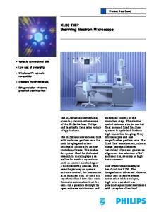
There is also a paper logbook at the SEM that users must fill out completely. It is for the purpose of recording the actual SEM use in order to help staff with problem solving as well as administrative details. This gives the staff archival information on what the tool is used for, how long it is to be used, who is using it, and for what subsystem. In addition, the blank Purpose/comments area gives you the space to tell the staff about SEM problems or remind you what you did during this SEM session, etc. Statements on what you were doing also help staff understand how the SEM is being used and enable better support. Figure 3 shows a sample log sheet. Return to STEP 2 Date ______________

Name _____________________________

Start Time_________

Circle Use: SEM

Finish Time_________

Sample__________________________

EDAX

EBSD

Supervisor _________________________________

STEM

Nabity Litho Bakscatter

Purpose/Comments:

Figure 3. Sample SEM log sheet kept at the SEM.

Sample Preparation Your sample can be mounted on one of a number of sample mounts. The simplest mount is the pin disc made of Aluminum and shown in Figure 4.

Figure 4. Simple SEM sample mount showing a metal sample attached with sticky conducting tape. The Copper tape affixed to the top of the sample insures a conductive path to ground for the top film, esp. if the substrate is an insulator. Also shown to the right is the removable Aluminum SEM sample Pin Mount. The large round table is the

Title: Scanning Electron Microscope Operation Author: Roger Robbins The University of Texas at Dallas

Page 10 of 72 Date: 6/22/2011

mounting platform that slides onto the SEM stage. The Allen wrench fixes the little sample mount stem to the mounting platform – do not over tighten.

Sample Holders There are a huge number of sample holder designs for SEM samples. We have a few, (Figure 5). However, for special sample configurations you should consider purchasing special sample holders that fit your needs, and most importantly, our SEM. Please consult with the Clean Room Staff SEM owner before ordering.

Figure 5. Sample holders in stock. These range from standard small pin mounts to edge profile holders to multiple pin to 4” and 6” wafer holders. There is also a transmission electron microscope sample holder (second from left on bottom row).

Sample Grounding The sample needs to be electrically connected to the sample holder to prevent the electron beam from “charging” the sample and distorting the image. This is usually done through conductive tape. We have double and single sided Copper sticky tape. If you have a conductive sample this simple attachment will work fine. If you have an insulator substrate with a conductive film on the top, the top film must be electrically connected to the Aluminum sample holder. This can be done with the Copper sticky tape looped around the edge to the top surface of your sample. If your sample is an insulator, then you may need to coat it with a conductive material – i.e. Au/Pd or Carbon. Title: Scanning Electron Microscope Operation Page 11 of 72 Author: Roger Robbins The University of Texas at Dallas

Date: 6/22/2011

Sample Coating Fortunately, we have a “Hummer VI” sputter deposition system1 located in Bay 5 just for this task. It has a Gold/Palladium target and a sputter deposition rate of about 1.2 Angstroms per second. Thus about 2-4 minutes of sputtering will apply enough metal to conduct the SEM electrons to ground and prevent charging without noticeably altering the topography of your substrate. The “Hummer VI” is shown in Figure 6. Note that if you coat an insulator substrate, you will need to connect the newly conducting top side to ground with a copper tape.

Figure 6. Hummer VI sputter deposition system for coating insulating SEM samples. Return to STEP 3

SEM Login You will have a user ID and password assigned to you after initial training. Thus when you arrive at the SEM, the screen will display a standard Microsoft Windows XP scene, waiting for you to execute the SmartSEM software. Click on 1

Thomas, Brian, “The Hummer VI,” www.utdallas.edu/Research/Centers/Cleanroom/Documents/eHummer.pdf , (10/29/2003) Title: Scanning Electron Microscope Operation Page 12 of 72 Author: Roger Robbins Date: 6/22/2011 The University of Texas at Dallas

the SmartSEM icon either on the left side of the left screen or the similar but tiny icon in the lower left taskbar of the right screen. This will bring up the Log On window in the left screen, Figure 7. Enter your username and password and click OK. This will bring up the Smart SEM software that runs the SEM.

Figure 7. Left screen Log On window. Note the ZEISS Smart SEM icon in the left column th 5 icon that calls up the log on window.

SEM Image Screen The next few steps of preparing the SEM for sample loading and image acquisition require commands from the software. The SEM user interface is spread across two monitors. The user interface screen is shown in Figure 8. The icons in the upper command line are used very frequently in operating the SEM and optimizing the image. The set of 6 tabs on the right side of the screen Title: Scanning Electron Microscope Operation Page 13 of 72 Author: Roger Robbins The University of Texas at Dallas

Date: 6/22/2011

contain command and parameter setting buttons for setting the SEM up for imaging. The row of icons at the bottom of the screen has commands allowing you to measure or label things on the image. The SEM image appears in the large region in the center. Return to STEP 4

Figure 8. User interface on the Left monitor after Log-On. Note the Imaging control icons in the upper row and the 6 tab command panel at the right side of the screen. Measuring and documentation icons are along the bottom. Also note the dual boxes at the upper left with Brightness = 44.7% and contrast = 36.3%; this is the handy HFP window that shows the value in % range of any adjustment knob on the keyboard. The strip of information at the bottom of the image frame is called the Data Zone and contains the micron bar, EHT, WD, etc – this strip is saved with the image.

One of the handiest tools hidden in the View menu is the Hard Front Panel option. If you pull down the “View” menu and click on the “Toolbars…” command, a new window will appear having an option for “HFP Status” with a check box next to it. Click in the box and close the windows. This will produce a pair of small window boxes with numbers in them. There will be a label assigning these numbers to a parameter pair such as Magnification/Focus which will correspond to the numeric value of the designated knob positions by (+/-) percent Title: Scanning Electron Microscope Operation Author: Roger Robbins The University of Texas at Dallas

Page 14 of 72 Date: 6/22/2011

travel from their origin. This conveniently gives you a numeric gauge for the amount of adjustment the knob is providing. If you grab the boundary of this window pair, you can move it to a convenient location in your user interface screen. This way, you will know how much magnification you are requesting, for example. The functions listed in the window match all the adjustment knobs on the keyboard and automatically appear when any of the knobs are just slightly touched.

Figure 9. Screen on the right monitor showing the Stage Manager, ChamberScope, RemCon32, and EM Server support windows open. This is a practical assortment of windows for safe operation of the SEM. Note the ChamberScope “Eye” icon at the lower left of the command line. NOTE: If you change this arrangement of windows during your SEM session, please put them back before you log out so the next user will have a standard display.

Sample Loading Now that the sample is prepared and mounted on the SEM sample mount, we have to vent the SEM to load it. This is done by clicking on the Sample Exchange icon in the upper left of the SEM image screen, Figure 8.

Title: Scanning Electron Microscope Operation Author: Roger Robbins The University of Texas at Dallas

Page 15 of 72 Date: 6/22/2011

This will turn off the SEM high voltage and in a little pop-up window ask if you have retracted all extendable probes – (EBSD, STEM, Backscatter detector) – so that the stage will not collide with them and damage the very expensive probes. Before clicking in the popup window, physically go look to see if the probes have been retracted – even if you “know” they have. These “probes” are generally worth as much as a mid-size Mercedes Benz! Make sure of their status. The stage usually vents in about 1 minute. When it arrives at atmospheric pressure, gently pull the SEM chamber door open with its handy handle. The stage table has a stainless steel disk at the center of a Copper table that has a bevel on its rim that fits the reverse bevel on the underside of the sample holder. Carefully slide the sample holder over this disk until it docks against the cross bar on top of the SEM stage table. Note that the sample holder copper docking disk underneath, has a flat side on it – this is the side that meets the docking bar on the stage table. Take great care in sliding this on or off because there are delicate mechanisms right next to the SEM table and on the stage. See the SEM stage in Figure 10. Return to STEP 5

Sample holder bottom. Beveled slot, flat end. Docking bar SS Docking Disk

Delicate electrical contact slider

Figure 10. SEM stage showing sample mounting table with small round docking disc and banking bar. Hand holding sample holder shows underside of holder with the reverse beveled slot and flat end that dock against the bar on the SEM stage table. Also note the delicate fixtures around the SEM stage table that can be easily damaged by a wandering thumb.

After the sample is properly mounted onto the SEM stage and inspected, gently close the chamber door. Just as it closes, it will “latch” closed by the force of a Title: Scanning Electron Microscope Operation Author: Roger Robbins The University of Texas at Dallas

Page 16 of 72 Date: 6/22/2011

magnet at the back of the stage so that the door will be held closed against the sealing O-ring when the vacuum pump starts, thus preventing an old problem of sucking room air into the chamber. Return to STEP 6

Now click OK in the box on the screen asking “Press OK to Pump.” The pump down sequence will take several minutes to achieve sufficient vacuum in the chamber for the system to open the column valve and establish a beam. In the meantime, you can click on the “Vacuum” tab in the right hand panel of the screen to view the vacuum level in the chamber and the gun. The gun should be below 8x10-10 Torr and the chamber vacuum line will be grayed out until the vacuum achieves a measurable level. The chamber will eventually achieve something in the low 10-6 Torr range. Return to STEP 7

Establishing the Electron Beam As the vacuum level in the chamber drops below 7.5x10 -5 Torr, the column valve will open and the gun EHT (High Voltage) will “Run Up.” By clicking on the Gun tab on the right side of the SEM screen, you can see the gun conditions. Normal operating conditions are shown in Table 1 below. Table 1 Normal Gun Conditions Parameter

Value

EHT

19.79 kV

Extractor V

4.40 kV

Extractor I

157 micro A

Fil I

2.410 A

Fil I Target

2.410 A

Extractor A Target

4.40 A

EHT Target

219.79 kV

If the electron beam has been on and at high voltage, the system will automatically bring it back on after proper vacuum levels have been reached. If the high voltage does not come back on, you can switch it Title: Scanning Electron Microscope Operation Author: Roger Robbins The University of Texas at Dallas

Page 17 of 72 Date: 6/22/2011

back on from the Gun tab window by clicking on the drop down menu under “Beam State=” and click “EHT On.”

Stage Control Now that a beam is established, the substrate needs to be positioned under the column so the beam can see it. This requires moving the stage from its default loading position to the inspection location which may depend on the sample and its size and shape. Before moving the stage, bring up the “Chamber Scope” window by clicking on the “Eye” icon at the lower left task bar of the right side LCD monitor. This will bring up a window into the SEM chamber viewed from the rear looking toward the front door. The image is an infrared image illuminated by 6 IR LEDs. Note that the image shows the stage in a mirror image presentation, since the video camera is mounted on the back wall of the chamber looking toward you. In any case, this allows you to see the mechanical movements of the stage in real time. This is important to help prevent collisions and improve the speed at which you can find your sample. By the way, the stage is electrically isolated and if there is a stage collision with anything inside the chamber, the SEM will very softly “Beep” and if the Sample Current Monitor is OFF2, then the stage motors will turn off at collision. If this happens and you know exactly why, you can manually back the stage away from the collision – if you are uncertain, please call the SEM staff person for immediate assistance.

Joystick Stage Control The stage movement is controlled manually by a dual joystick desk console shown in Figure 11. In general, the LEFT joystick controls the Zaxis movement and the stage tilt angle, and the RIGHT joystick controls the X, Y motion and the stage rotation – “5-axis stage.”

2

NOTE: The Sample Current Monitor (SCM) should always be “OFF” unless the user is actively measuring the sample current. Title: Scanning Electron Microscope Operation Page 18 of 72 Author: Roger Robbins Date: 6/22/2011 The University of Texas at Dallas

Figure 11. Joystick Stage control. LEFT stick performs stage Z-travel and Tilt: Z-travel – push lever up or down; Tilt – push the lever right or left. RIGHT joystick moves stage in x and y and twisting the right stick causes the stage to rotate.

To raise the stage into the ChamberScope view, push upwards on the LEFT joystick – stage speed is controlled by the amount you push the stick upwards. The stage will travel “up” in Z and the ChamberScope will show its rise. Release the joystick to stop motion. Note that the z-axis velocity is also governed by the image magnification: If the magnification is high, the stage moves very slowly, if it is low, the stage moves fast. When the stage rises to within about a centimeter of the bottom of the conical lens as seen in the ChamberScope, stop. The (x,y) position can then be adjusted with the RIGHT joystick so that your sample is under the electron lens. Note that the stage (x,y) center is about (65,65) mm. If your sample is at the center of the stage, then just move the stage to these coordinates and adjust around the center to find your exact target. Tilting the stage is effected by tilting the LEFT joystick to the left or right. This also means that while you are raising the stage in the z-axis, and if you also push the joystick right or left, the stage will simultaneously tilt. Watch out for this dual motion (via the ChamberScope) to avoid awkward stage conditions. The stage will only tilt toward the detectors on the left side of the SEM chamber, (which is to the right in the ChamberScope view because the video camera is looking at the stage from the back wall of the SEM chamber). If you reach the tilt limit, the SEM will stop tilting the stage and show an error “TILT LIMIT.” By the way, if you run into a stage limit error, just push the lever in the other direction to move away from the limit. Nevertheless, the correct initial direction to push the tilt stick is to your right. You can observe the exact tilt angle in the window executed by the “Stage” tab on the SEM Control panel to the right of the SEM image screen. See Figure 9. This Stage Control window is opened under the Stage command menu in the upper left screen command line. Title: Scanning Electron Microscope Operation Author: Roger Robbins The University of Texas at Dallas

Page 19 of 72 Date: 6/22/2011

The RIGHT joystick (x,y,theta) works the same as the LEFT joystick: the more tilt you give the joystick, the faster the stage moves. Also, if the magnification is high the x,y motion is slow and vice versa. Stage rotation is effected by twisting the RIGHT joystick handle one way or the other. Twisting the handle to the right, (clockwise) will cause the stage to rotate about stage center in a clockwise direction. If your target is far away from the stage center, it will appear to translate off the screen because this rotation center is independent of your sample location.

Note that x and y movements can be somewhat confusing because there may be as many as four or five independent coordinate systems involved in the movement. For example: Substrate coordinate system, Stage coordinate system, Beam coordinate system, Joystick coordinate system, Chamber Scope coordinate system, and a software coordinate compensation interpretation system that tries to make user sense out of all the above complications. 

Digital Stage Control If you open the Stage Manager window and place it in the right screen then you will see two sets of coordinate values for each of the stage coordinate axes. The right hand column is a command listing and if you double click in a coordinate box, you can type in a coordinate number, hit enter, and the stage will move to that coordinate value. It will move fast – not coordinated with the magnification – so this method of moving the stage loaded with danger of collision! I recommend that an operator never use this method for moving the stage up to operating height from the loading position – always use the joystick while watching the video camera. The real value in being able to load stage coordinates comes after the stage is in position under the objective lens and the stage needs to be driven in x and y to a known or mapped sample location.

Coordination of Stage and SEM Image Movement Because of the multiplicity of coordinate systems and apparent conflict of motions, there is an easy way to coordinate the motions of the SEM Image, the Joystick motion and the stage motion in the video camera image. On the SEM Keyboard there is a knob entitled Scan Rotation. If we set this to 90 degrees, then the SEM image, the joystick and the stage as viewed in the video camera image will all move in the “same” direction according to the operator perspective. To do this we will need the “Hard Front Panel” option active. This pair of windows will show the exact value of each of the knob settings and will change to Title: Scanning Electron Microscope Operation Author: Roger Robbins The University of Texas at Dallas

Page 20 of 72 Date: 6/22/2011

which ever knob we turn. To set the 90 degrees simply turn the Scan Rotation knob until 90 deg shows in the window. Return to STEP 8

SEM Keyboard Before we discuss finding the sample, we need a short overview of the SEM control keyboard, Figure 12.

Figure 12. Picture of the SEM console keyboard. This console contains a standard (laptop) style keyboard layout in the midst of a number of knobs. The knobs perform repetitive and sensitive operations of SEM control such as focus and magnification among many others.

The SEM keyboard has a number of knobs to give the operator analogue-like control of SEM parameters. The large knob on the left is magnification and the large knob on the right is focus. The two knobs on the upper right are brightness and contrast. And the two knobs on the upper left are stigmators. These are the most used knobs and their functions require frequent, precise analogue adjustments to achieve visible optimization of image quality. The lesser used knobs will be described later. These give the more experienced operator the ability to operate the SEM much faster.

Finding and Positioning the SEM Image Title: Scanning Electron Microscope Operation Author: Roger Robbins The University of Texas at Dallas

Page 21 of 72 Date: 6/22/2011

Sometimes the SEM will start scanning but the screen will be totally dark. How would you find an image from this condition? The normal way would be to reduce the magnification to minimum, and turn up the contrast knob on the SEM keyboard. This will usually bring up a gray scanning field with some fuzzy bright spots in it. If your stage location has been centered (at 65 mm in x and 65 mm in y) and your target sample is at center and about 1 cm below the tapered end of the objective lens, the fuzzy image will show an out-of-focus image of your sample and perhaps some stage parts. Slowly turn the Focus knob on the keyboard to the right (clockwise) to lengthen the working distance – (distance between the lens and the beam focus point in Z). Soon your image will begin to come into focus. Now you can position the stage in (x,y) and working distance (z) appropriate for the sample.

Multi-Sample Holder Map When you are using the multi-sample holder, this step appears to be a troubling conundrum for new students trying to find the location of each of the samples, (Figure 13). The reason that there is difficulty in this task is that the default coordinate system of the SEM image on the left screen is at 90 degrees from the motion actuated by the joystick and seen in the video camera image of the stage motion in the Chamberscope screen. Also the Chamberscope camera is looking at the sample from the back wall (invoking a left-right reversal) and at a shallow angle so that it is hard to tell where the stage is located in the front-back direction.

Figure 13. Photo of the rectangular multi pin sample holder.

To compensate for this confusion and perhaps speed up the effort locating a sample, I have created a coordinate location map that sets coordinate Title: Scanning Electron Microscope Operation Author: Roger Robbins The University of Texas at Dallas

Page 22 of 72 Date: 6/22/2011

locations for all four corners and each of the 12 pin mounts. This data is only valid if the stage rotation is set to 0 degrees and the sample is mounted on the holding button with the banking bar on the left side of the table as one loads the rectangular multi-pin sample holder onto the SEM stage. The Pin number is the stamped number on the holder as seen in Figure 13 and Figure 14.

SEM Stage Coordinate Location of Multiple Pin Samples

Y

X

23 43 49

29

44

59

74

1

2

3

4

64

5

6

7

8

79 85

9

10

11

12

87

*Red numerals identify Sample location marks. **Read Table for Sample 6: Stage Location = (64,44) millimeters. ***Upper Left corner: Location = (43,23) millimeters. ****Table values are only valid for stage rotation set to 0 degrees. *****Corner number related to sample positions Figure 14. Map of pin locations with stage coordinates. Also including corner locations for finding edge profile samples taped to the sidewalls of the holder.

The significance of the Corner Coordinates is that if you are looking at multiple cross section samples taped to the side of the sample holder, you can use the corner values as starting points to find your samples. Then you can move the stage and view samples in a row by moving the SEM image with the Joystick along one axis.

Title: Scanning Electron Microscope Operation Author: Roger Robbins The University of Texas at Dallas

Page 23 of 72 Date: 6/22/2011

Scan Rotation Coordination with Stage Motion One more trick can be invoked to make finding things easier. If you set the rotation angle of the electron beam (Scan Rotation) to 90 degrees, then the movement of the SEM image in the left screen will correlate to the apparent motion of the stage in the right hand screen in the Chamber scope window. (Of course the joystick (x,y) coordinate system will translate to (+x=+y’) and (+y= -x’) where the primed coordinates are the “Stage Manager” coordinates). Setting the Scan Rotation is effected by rotating the Scan Rotation knob on the keyboard and noting the scan angle from the knob readout boxes (“Hard Front Panel”) at the top of the SEM image window on the left screen. The 90 degrees scan rotation causes the electron beam scan to rotate from the horizontal direction to the vertical direction as it scans across the sample but is unchanged in the screen image – this consequently causes the SEM image to rotate 90 degrees.

Stage Motion Warning Note again that moving the stage using the command boxes in the Stage Manager windows is loaded with danger – you need to make sure that the stage will not hit anything along the way to the new coordinates you type into the command windows. Also make sure that the Specimen Current Monitor is “OFF” at all times during stage movement. This gives a small amount of insurance against catastrophic damage if the stage does hit anything in that the collision sensor will turn off the motors upon contact – but not if the current monitor is “ON”.

Image Positioning Shortcut There is another really handy feature of this SEM software that remarkably speeds up the positioning of the sample for a photo. This is needed principally because as you increase the magnification, the portions of the image outside of the center region of the image on the screen expand and move off screen. So after you have obtained the SEM image of your sample by using this handy trick, you can drive a specific spot on the image to the center of the screen where a magnification change will not move it again. This is accomplished by sequentially holding down the “Ctrl” key and then pressing the “Tab” key on the keyboard. This action causes a big green crosshair to appear on the screen. Move the crosshair with the mouse to the location in the image that you want centered in the screen and click the left mouse button. The SEM then either moves the stage or the beam, depending on the magnification, so that the image at Title: Scanning Electron Microscope Operation Author: Roger Robbins The University of Texas at Dallas

Page 24 of 72 Date: 6/22/2011

the crosshair moves to the center of the screen. This is a magnificent tool to speed operation. Return to STEP 9

Focus and Stigmation To sharpen the nominal low magnification focus used to find the sample, gradually increase the magnification and select successively slower scans to decrease the image noise (snow). If the image feature moves offscreen as you increase the magnification move it back onto the screen with the (x,y) joystick or the neat shortcut outlined in the previous paragraph. As the magnification increases and fine details come into view, select the “Reduced Raster” button at the top of the screen. This will bring up a small, size-changeable active box on the image that displays a small portion of the SEM image. This allows you to switch to slow scan to bring out sharp details but simultaneously increase the frame rate to make it easier to observe the image focus in relation to focus knob changes. Click on scan rate icon #4 to obtain the best image to focus at high magnifications. You can now further increase the magnification to finely focus the image. Focus technique requires astute observation of the degree of “fuzziness” in the image. However if you turn the focus knob until the image goes distinctly out of focus, note the knob position, and then turn the focus knob the other way until the focus is distinctly out of focus by about the same amount as the previous position, then focus will be about in the center of the two knob positions. Turn the knob back to this center position and proceed to further increase magnification. If the image is again fuzzy, repeat the focus adjustment until the focus is clear. Stigmation is observed as focus distortion in the image which gives the image a directional fuzziness. This occurs because the electron beam cross section is shaped oblong like an ellipse when it is stigmatic. The axis of the oval spot can be in any orientation and the result is that edges of the image parallel to the long axis of the elliptic spot are sharply focused and the perpendicular image edges are fuzzy and axially stretched. This gives the image a uniform fuzziness orientation.

Figure 15. Example of opposite astigmatism orientation on either side of center focus (Left and Right images), and fuzzy center focus due to residual astigmatism at focus. Astigmatism correction is the next step to clear the fuzziness at focus. Title: Scanning Electron Microscope Operation Author: Roger Robbins The University of Texas at Dallas

Page 25 of 72 Date: 6/22/2011

To correct astigmatism, rotate one of the stigmator knobs until the fuzziness increases noticeably and then rotate it the other way until the fuzziness again increases. The proper stigmation correction position is in the middle of these two extreme knob positions, (See Figure 15). Repeat this approach with the other stigmator knob, and then refocus with the big focus knob. This should bring the image to a sharp focus and you are done. So now that we have covered the manual focus procedure, the SmartSEM software in some cases can make this an effortless button-push procedure. On the row of icons at the top of the screen, Figure 16, is a special “Auto Focus + Stigmate” function that is activated by the middle mouse button (Roller wheel). By clicking on this icon with the roller wheel on the mouse, the system will snap into an auto focus mode where the scan is reduced to a small rectangle in the center of the image and a window with a progress bar pops up showing you the focus status. Allow this to complete and observe the results in your image. The little focus and status box will disappear when the function is complete. If the image has sharp details, the auto function was successful. If the image appears way out of focus, it got lost. So the auto focus function depends on the target to have sharply contrasted features to be successful. If the image is low contrast, the auto focus function can twiddle until it is lost and you will have to manually re-focus. Practice is required to improve your skill at this focus task.

Figure 16. This is the panel of action icons at the top of the SEM image page. The third icon from the right is the auto-focus button. The numbered boxes are standard scan rates. Button #1 is used for finding the image and stage movement, Button #2 for stage movement, Button #3 for focusing, Button #4 for image capture, and Button #5 for image capture. Return to STEP 10

Aperture Align Any time a different aperture has been selected, the beam needs to be realigned. After you establish focus at a reasonably high magnification (>20KX), click on the “Aperture” tab in the menu set at the right of the SEM image window. Then click on the “Focus Wobble” command and set the “% Wobble” to about 5%. This will automatically change the focus +/5% in a repeating fashion. The image will appear to go in and out of focus as well as oscillate in its position. Your task to align the beam to the Title: Scanning Electron Microscope Operation Author: Roger Robbins The University of Texas at Dallas

Page 26 of 72 Date: 6/22/2011

aperture is to adjust the x and y “Aperture” knobs on the keyboard until the image does not move (wobble) any more – it should just go in and out of focus in the same location. When you have stabilized the image wobble just click on the “% Wobble” command and it will stop. Then repeat the focus and astigmatism correction. Brightness and Contrast The gray level and contrast of the image are set by the two knobs on the upper right corner of the keyboard. The concept in setting these parameters is to have a brightness level that shows dim objects, but a contrast level that avoids white saturation. Contrast also determines the edge definition of objects when looking for sharp, high contrast edges. Electrically, the brightness knob sets the zero offset of the gray level and the contrast knob sets the gray level gain. These knobs are linear in effect, but affect each other – i.e. increasing the contrast makes the image brighter, but so does the brightness knob.

Figure 17. High contrast image with saturation (Left), Normal image, (Center), Low contrast image (Right).

Scan Speed Scan speed is an important parameter with many ramifications. In general, for a fast scan speed, the image contains more noise (snow), and for a slower speed, the image becomes less noisy and more highly resolved. However, the fast scans reflect real time movement of the stage better than the slow scans. This gives the operator an easier view of stage movement and allows a faster positioning ability. Because the SEM imaging technique is inherently slow, any speed improvement will become highly appreciated by the operator as experience level increases. When the stage is positioned with the desired image in position, the scan rate can be slowed to set the focus and reduce noise for image capture. The software can be trained to automatically impose the fast scan if you move the stage. This command is found in: “Tools\User Preferences\stage\Fast Scanning\ (ON or OFF).” Title: Scanning Electron Microscope Operation Author: Roger Robbins The University of Texas at Dallas

Page 27 of 72 Date: 6/22/2011

There are other digital manipulation techniques to reduce noise in the image. Under the scan tab there is a box that allows the user to choose various noise reduction methods such as pixel averaging, frame averaging and the extent of averaging. In the pixel averaging technique, the SEM captures a settable number of brightness samples at each spot the electron beam moves to in a frame, then averages them all together and displays the spot as the average. This technique reduces the image noise by reducing the spot noise at each spot and results in a real time moving image if the stage is moving. The frame averaging sweeps an entire frame, stores it, and then averages it with the next frame for a selectable number of frames. This creates a dynamic image that produces ghost images for a moving stage that slowly coalesce into the final image when the stage stops moving – not so useful for motion situations. Return to STEP 11.

Image Capture Image capture is accomplished by “freezing” the image (at the “End of Frame”)3 and clicking on the Microsoft “File” menu at the far upper left of the screen. This brings up a reduced size window with commands to save the image, Figure 18.

Figure 18. Image capture screen.

To save an image with support data, select your directory by clicking on “Change Directory” and selecting your directory. It will nominally default to your assigned directory on the D: drive, but if you want to store directly to 3

Set “Freeze on end of Frame” by opening the top row “Scan” Menu and selecting “Freeze on End of Frame.” Title: Scanning Electron Microscope Operation Page 28 of 72 Author: Roger Robbins Date: 6/22/2011 The University of Texas at Dallas

a memory stick, you will have to select it. Type in the name of the image file you want to store. Click a check mark into the box titled “Annotation” to save any screen text annotation with the image. Fill in any special text explanation you want to save with the file into the “User Text” box. This text will save into the image file so that you can see it in a directory listing but will not imprint on the image.

Special Imaging Techniques Charging Many times during your career at the SEM, occasions will arise when you would like to image an insulator material. Unfortunately, SEM physics objects to that… If you were to try to image an insulator, the image would appear to contort into strange conditions of brightness, shape, and auroralike movement. This would be due to electrons congregating in ever larger numbers on the surface or body of the insulating substrate, thus building up a space charge which severely affects the electron beam. This phenomenon can cause many strange and dynamic effects in the picture too numerous to describe here.

Figure 19. Examples of objects charging in SEM

To avoid charging, we normally sputter coat substrates with a very thin film of Gold and Palladium mix1 so that the coated surface will be able to discharge excess electrons to ground and thus not cause the imaging beam difficulty. Charging in a sample is highly complicated and depends on many things, but the balance of electrons hitting the target and those escaping the target is the key to controlling the consequences. Ideally the sample potential should remain at ground level. The potential above the sample is set by the voltage of the substrate and as electrons from the beam enter this field, they are deflected. This can shift the beam and thus move the SEM image. Title: Scanning Electron Microscope Operation Author: Roger Robbins The University of Texas at Dallas

Page 29 of 72 Date: 6/22/2011

In some cases you might be able to take advantage of a physical characteristic of electron collision with a tilted surface to help balance the incoming electron charge with the electron charge leaving the surface via scattering. From the data in Figure 20, you can see that as the sample surface is tilted more parallel to the beam, setting a shallow grazing angle, that more electrons scatter out of the surface. If the substrate drain path current can be balanced with the escaping electron charge rate, then the surface could be brought to neutral voltage and the image would become non-charging. Figure 20. Backscatter electron emission as a function of substrate angle with the primary Other things can happen on a beam. This shows that as the angle between electron beam and the surface tilts, more more local basis as electrons the electrons escape. (Data from Kanter, H. are captured in local regions. (1957)).

These regions will cause the SEM image to “blossom” into bright, random shaped phantom objects in the picture due to clouds of excess electrons bleeding off of the surface and entering the electron detector signal. Many other consequences can also happen, but they all prevent a true image from being captured. Therefore considerable effort is required in some cases to prevent charging. Electron Penetration Effects The SEM imaging technique sometimes determines whether you can see the aspects of your substrate that you are interested in. For example, if you need information from the topography of the sample, you should consider the penetration depth of the probe electrons. As electrons enter the sample surface, they penetrate into the body of the material a distance depending on several parameters, chiefly the energy of the electron itself and the material. The deeper they penetrate, the less surface information is contained in the image, and the more material parameter information they convey. However, the higher energy electrons produce a higher geometric image resolution. This occurs because higher energy electron beams are distorted less by the SEM hardware than lower energy beams. Therefore you will need to find an appropriate compromise to meet your requirements. Title: Scanning Electron Microscope Operation Author: Roger Robbins The University of Texas at Dallas

Page 30 of 72 Date: 6/22/2011

Backscattered Electron Image By collecting mostly backscattered electrons from elastic collisions with atoms in the substrate, you can obtain an image with contrast more from the material type than from the topography, (See the topic of Backscatter Electron Detector). Figure 21 shows a graph of backscattering coefficient as a function of Z (Atomic Number). As the atomic number goes up, the material becomes more efficient at producing inelastically backscattered electrons which can be captured by backscattered electron detector. This will produce an image with material contrast where material consisting of heaver atoms show up as brighter regions ions in the image.

Figure 21. Electron backscatter coefficient vs. Atomic number, Z. This characteristic increase in electron emission with Z creates image contrast in Z, or “mass contrast.”

Secondary Electron Image The standard SEM image is generated by “secondary’ electron emission from the substrate. These are low energy electrons (less than 50 eV) produced both by the primary electron beam and the high energy backscattered electrons. However while the primary electron beam can Title: Scanning Electron Microscope Operation Author: Roger Robbins The University of Texas at Dallas

Page 31 of 72 Date: 6/22/2011

penetrate the substrate by several or many microns, the escape depth for the secondary electrons is only on the order of tens or hundreds of angstroms. Thus they are generated very close to the surface, (Figure 22).

Figure 22. This schematic depicts generation of secondary electrons near the surface from the primary beam and backscattered electrons.

To the first order, the energy distribution of the secondary electrons is independent of the energy of the primary beam. Because of this characteristic, a “universal” curve can be generated for all metals, Figure 23. The curve rises from a zero emission coefficient for zero secondary electron energy, to a peak between 1.3 and 2.5 eV for most metals, and then falls to a low value for secondary energies greater than 10 eV. For insulators, the peak falls at a lower secondary electron energy, because there is a lower potential barrier at the surface of insulators than there is with metals, and this allows a larger number of slower secondary electrons to escape. The SEM video system produces a brighter pixel where the secondary electron current striking the electron detector is greater.

Title: Scanning Electron Microscope Operation Author: Roger Robbins The University of Texas at Dallas

Page 32 of 72 Date: 6/22/2011

Figure 23. This graph shows the envelope of probabilities of secondary electron escape from the surface of metals as a function of the secondary electron energy. The data shows a probability of escape peak between 1.3 and 2.5 eV. This peak denotes the general energy level of the secondary electrons.

This data sets a value for the energy of the secondary electrons collected by the secondary electron detector in the SEM. Thus the EverhardThornley electron detector with its collection grid has to accelerate the secondary electrons to several hundred eV to cause a phosphor photon to be generated and then converted to an electron current that is multiplied many times by the photo multiplier and video pre-amp. It is this current that produces the standard SEM image on the computer screen.

Image Storage Note that even if you save your images onto your assigned disc space on Drive “D:” on the SEM computer, it is subject to removal without notice by staff. This must be because if the disc becomes full, then the operation of the SEM is compromised and the Clean Room Staff needs to be able to restore operation by removing files. Therefore, it would be prudent to save your images to a memory stick instead of the SEM hard drive. Normally images would only be removed if a problem arose with the SEM operation. But you don’t know when that will happen and you wouldn’t want to lose critical information. Return to STEP 12

Sample Removal Sample removal is accomplished by clicking on the “Specimen Change” icon at the top left of the SEM image screen. This action will automatically turn off the high voltage and close the column valve before venting the chamber. Before you click on this icon, please manually drive the stage down in z to a height of 10 mm, then move the stage in x and y to the center at (65,65) mm. for the x,y move you can type into the “go to” box in the stage manager menu the Title: Scanning Electron Microscope Operation Author: Roger Robbins The University of Texas at Dallas

Page 33 of 72 Date: 6/22/2011

65,65 locations for an auto drive move. This will move the stage to a safe position in a safe manner so that there will not be any collisions during the move or the door opening action. When you remove your sample and click on the ensuing “Press OK to Pump” button on the popup window, the SEM will re-establish vacuum and bring up the High Voltage (EHT). If you are finished, follow the EHT Shutdown Procedure in the next section. Return to STEP 13

Shutdown Procedure If you are done and ready to leave, remove your sample and pump down the sample chamber. When the pump down starts, you can log off to end your session and sign out of the logbook. The EM Server program will take care of the SEM hardware after you log out. The logoff will stop the use timer and log you off so that the tool is ready for the next user. At logoff, the high voltage for the gun is automatically shut down. This will preserve the life of the field emitter tip that produces the electron beam. It is expensive – many thousands of dollars.

Completion Check List [Before leaving SEM, set the machine to its standard idle configuration mandatory.]

Job Completion Checklist 1 2 3 4 5 6 7 8

EHT off Return software to standard SEM configuration Remove Sample Re-establish vacuum Log out of SEM software Complete Log Book entries Make sure that the SEM table is clean and free of samples Return tools to tool home

Title: Scanning Electron Microscope Operation Author: Roger Robbins The University of Texas at Dallas

Page 34 of 72 Date: 6/22/2011

Rules of SEM Operation The official rules pertaining to time, cost, and operation follow: Time Allocation: Because this tool is a high use system, we have established a sign-up protocol to ensure that the tool is used fully and to alleviate schedule overlaps and conflicts on the UTD web page, o [ http://www.utdallas.edu/~hcf011000/cgi-bin/Login.pl ] o There is an SEM time allotment page that you can log in to and capture time on the machine. o Users are permitted to sign up for 10 prime time hours per week (Prime time hours are Monday – Friday 8:00 AM to 6:00 PM). o Signup times are set at 1 hour time blocks (min time allowed). o Users are charged for the time they reserve the tool for unless they cancel at least 24 hours before the start of their session. You may swap time with another user if necessary. o Non prime time hours (Weekends and weekdays from 6:00 PM to 8:00 AM) have no restriction on the length of signup time. Fill out the logbook at the start of your session. Do not store or leave samples at the machine. Samples can be thrown away by staff without notification. Do not use SEM computer to check e-mail or browse the internet or play games. Specimen current Monitor (SCM) should be OFF at all times except for the short time it takes to measure specimen current. Never unplug the Pico Amp Meter cable from the front door while the electron beam is on – stage could charge up to thousands of volts and zap the pico ammeter when the cable is plugged back in. You will be given a password after your specific training on the SEM. If you sign up, you are expected to keep your appointment with the SEM. Remember, the current rule is that if you sign up you and you need to cancel, you must cancel 24 hours before your scheduled time. This means that if you sign up the day before, and discover you can’t make it, you may pay for the time anyway – unless you make arrangements with another user to take your place and make note of that in the logbook at the reserved time slot. The person taking your time must sign in the paper logbook for the time used.

Standard Configuration When you complete your operation, return the machine to standard SEM configuration. If you have been trained on one of the several subsystems and you leave the tool set up for that system, the common SEM user may not know how to return to the standard operation.

Title: Scanning Electron Microscope Operation Author: Roger Robbins The University of Texas at Dallas

Page 35 of 72 Date: 6/22/2011

Remove Sample When you complete your time on the machine, remove your sample. Also whisk your sample away from the SEM – don’t leave it lying around on the table, etc. It will be subject to destruction by the staff cleaning up the table.

Logbook Fill in the logbook. If you leave blanks, you could be subject to denied use of the SEM. Purpose/Comments The Purpose/Comments section in the logbook is intended for recording what you did and note any problems encountered. This is helpful to staff in diagnosing problems and noting what type of work is done in the SEM for logistic support data. Please fill this in!

Consolidated SEM Operation Instructions This is an abbreviated list of operating instructions that guide you through the “what to do next” confusion that may ensue after initial training for a new user or an encounter with the SEM after a long absence from SEM operation. It is essentially a step-by-step listing of the operating sequence tasks with reference links to the full explanation in the instruction sections in case the abbreviated listing does not trigger full understanding. In this list of operating steps, there will be a blue “Jump to” word that you can click on and the document will jump back to the full explanation section. When you finish reading the explanation, click the blue “Return to Step n” link and the document will return you to the Consolidated Instruction step that you started from. STEP 1. Schedule SEM time on-line. STEP 2. Fill out paper Logbook at the SEM.

Jump to:Time Scheduling

Jump to logbook

STEP 3. Prepare Sample (Cu Tape, Hummer Au dep., Size sample, etc. …can be done before scheduling SEM), and Mount Sample on Pin Mount Jump to Sample

Title: Scanning Electron Microscope Operation Author: Roger Robbins The University of Texas at Dallas

Page 36 of 72 Date: 6/22/2011

STEP 4. Log-in to SEM software

Jump to Login

STEP 5. Vent SEM sample chamber.

Jump to Loading

STEP 6. Open door and mount sample on stage.

Jump to Loading

STEP 7. Close door and pump down chamber.

Jump to Loading

STEP 8. Position stage under objective lens with joystick – watching stage in the Video window. Use joystick to raise stage to focus point to avoid collision with lens. Jump to Stage Control

STEP 9. When system is ready (Scanning operational at EHT), drive stage to target location at low magnification. Jump to SEM Image

STEP 10. Focus and correct astigmatism. Jump to Focus

STEP 11. Optimize image (brightness, contrast, scan speed). Jump to Brightness

STEP 12. Capture image to Disc. Remember the strange rule that Staff has the power to erase any data that they need to without notice to the owner, so transfer your images to a memory stick before leaving. Jump to Image capture

Title: Scanning Electron Microscope Operation Author: Roger Robbins The University of Texas at Dallas

Page 37 of 72 Date: 6/22/2011

STEP 13. Exchange Sample (Vent, open door, change or remove sample, close door, pump down chamber). Never leave sample chamber at atmospheric pressure for very long. Jump to Sample Removal

STEP 14. Log-Off SEM software to stop your session cost timer.

STEP 15. Log out of Logbook. STEP 16. Clean up the SEM and the sample prep table. Note that Staff can toss your samples if they are left on the table.

Title: Scanning Electron Microscope Operation Author: Roger Robbins The University of Texas at Dallas

Page 38 of 72 Date: 6/22/2011

Operating Instructions for EDAX Material Identification System Introduction [Note that this is the detailed description section for operating the SEM/EDAX imaging system.] The “EDAX” system (Figure 24) mounted on our Supra-40 Scanning Electron Microscope is an X-Ray analysis system capable of producing an energy spectrum from X-Rays emanating from a specimen material that is struck by energetic electrons and analyzing the data to determine what elements are producing the X-rays. This principle is termed Energy Dispersive (X-ray) Spectroscopy (EDS). It is a type of X-ray Fluorescence Spectroscopy. The EDAX X-ray detector is a Lithium Drifted Silicon detector. To avoid Li migration under the influence of bias and temperature, the detector is chilled to liquid nitrogen temperatures. If the liquid nitrogen evaporates and the detector warms up above a threshold set in the software, the detector is turned off to reduce the bias to zero. This helps prevent deterioration of sensitivity because of the thermal and bias drift of the Lithium impurities. Filling the LN2 Dewar is a responsibility of the Clean Room staff. If you find that the Dewar is empty, ask a staff member to fill it. It will take at least an hour before the sensor is stable enough to capture reliable data.

Figure 24. EDAX LN2 Dewar and pre-amplifier mounted on the Gemini electron microscope column.

Title: Scanning Electron Microscope Operation Author: Roger Robbins The University of Texas at Dallas

Page 39 of 72 Date: 6/22/2011

Basically, the X-ray emission is stimulated by electrons from the SEM electron beam striking atoms in the sample material and knocking out inner shell electrons and creating electron holes where the ejected electron used to be. Then another electron from an upper shell of the same atom “falls” into this hole and liberates a photon having energy equal to the difference between the falling electron’s home level and the lower level it falls into. The energy of this liberated photon is in the range of X-ray photons; Figure 25.

Figure 25. Sketch of atomic energy levels and x-ray photon generation from SEM electron bombardment excitation.

By counting and sorting each X-ray into software bins according to the energy level of each X-ray, a graph can be fashioned that shows X-ray counts vs. energy (Figure 26). This results in a spectrum characteristic of the quantum energy differences in the electron energy structure of the atoms in the sample material. This spectrum can then be analyzed by the software and the elements contained in the material can be identified. With more analysis, the ratio of elements can also be identified. This document is intended to convey operating instructions to perform elementary material analysis at a basic level. It follows the step by step procedure for obtaining the data and generating a simple analysis. Students must obtain Staff training on this tool before attempting operation. The directions in this section assume that you have been trained and have some experience running the SEM itself.

Title: Scanning Electron Microscope Operation Author: Roger Robbins The University of Texas at Dallas

Page 40 of 72 Date: 6/22/2011

Figure 26. Example of EDAX spectra: X-ray counts vs. X-ray energy. The pattern of energy levels is analyzed to determine what element emitted the X-rays.

Starting Check List [Before using the system, determine what condition/configuration the SEM/EDAX is in – it should be in a standard state. List critical items that must be checked before operating SEM/EDAX.] 1. Check the LED status indicator on the back of the EDAX preamplifier box just under the big liquid Nitrogen Dewar. If it is red, the sensor is warm and needs LN2 added to the Dewar. If it is green, all is well. If it is not lit then the power is not on – activate the EDAX software and recheck. 2. How do you tell if the LN2 tank is empty? There are several tell-tale observations that suggest that the tank is empty and the sensor is warm: 1. Lift the lid at the top of the EDAX LN2 tank – if it is freezing cold and steaming, then it is likely there is still LN2 in the tank. 2. If the EDAX Genesis program sees no x-rays then it is likely that the X-Ray detector is shut off because it is above the operating temperature limit. 3. If the “Status” LED on the upper end of the EDAX signal amplifier at the base of the LN2 tank is illuminated in Red the amplifier is turned off because the temperature is out of spec.

Title: Scanning Electron Microscope Operation Author: Roger Robbins The University of Texas at Dallas

Page 41 of 72 Date: 6/22/2011

EDAX Spectral Analysis Setup Procedure [Detailed operating procedure from the perspective of a new operator.] Scheduling the tool This tool falls under the SEM scheduler at the following web site: http://www.utdallas.edu/cgi-bin/cgiwrap/hcf011000.Login.pl To get started on this scheduler, you must create an account following the link on the web page. Additionally you must have turned in an application form and have been given permission to create a schedule. Ask staff about this if you need further information. The time you reserve on the scheduler is used to calculate the charges your supporting project is charged for your time on the SEM. Fill out Logbook The paper logbook sitting on the SEM table must be filled out completely. Sample Loading Sample loading is similar to the SEM loading procedure. The only difference from the SEM procedure is that the Working Distance (WD) for the EDAX should be set to 8 mm in order to optimize the capture of the Xrays emitted from the sample. Finding Image Follow the standard SEM imaging procedure to find a standard resolution image and focus on the region of interest for EDAX analysis. See the section on SEM imaging. Establishing X-ray Capture

Setting Working Distance To set the working distance, double click on the Working Distance (WD) label in the Data Zone at the bottom of the SEM image screen. A small window containing the current working distance will pop up and allow you to type in 8 for the new WD. This will more than likely throw off the focus you have already established, so manually (joystick) move the sample stage up or down to bring the focus back. When you achieve reasonable focus with the stage movement, you can perform fine adjustment with the focus knob.

Title: Scanning Electron Microscope Operation Author: Roger Robbins The University of Texas at Dallas

Page 42 of 72 Date: 6/22/2011

Beam Energy If you know what elements to expect in your sample, look up the EDAX voltage on the wall chart for the K, L, and M shell electrons for the sample atoms and determine the highest energy of all elements in the sample. Then set the electron beam voltage (EHT) at twice the highest electron binding energy – limited of course by the 30 kV max beam voltage.

Turn off Chamber LED Illumination Before executing the EDAX software, you must turn off the LEDs that illuminate the interior of the stage vacuum chamber. The light from these LEDs causes the X-ray detector to count large numbers of phantom Xrays, and confuses the energy calibration. You can turn off the LEDs by sliding the illumination slider at the top of the Chamber Scope window all the way to the left. The screen will go totally dark. If after that, the window still shows a small spot of light, it indicates that the stage End of Travel Sensor is illegally active. The only way to cure this is to re-initialize the stage, which consequently requires re-establishing the SEM image at your target.

Illumination Error Recovery Recovering from the Stage End-of-Travel-Sensor illumination error requires re-initializing the stage. To do this, manually drop the stage back to a safe distance from the objective lens (Z~10 mm) and then open the “Stage” menu from the top row of command menus. Find the Initialization command at the top of the list and click on it. This will cause the stage to automatically drive to the zero end of each axis and reset the stage zero location. When it finishes this operation, it will have turned off the end of travel sensor illumination. This fixes the interference with the X-Ray detector and the EDAX system can work now. However, you have to move the stage to the previous location and find the spot on your sample that you want to record a mass spectrum from. WARNING: Please do not drive the stage in Z by inputting numbers into the digital move boxes – move it manually while watching the video camera so that you won’t hit anything.

Aperture Selection The beam current in the Zeiss Supra 40 SEM is set by choosing different sized apertures. The EDAX signal is more dependent on beam current Title: Scanning Electron Microscope Operation Author: Roger Robbins The University of Texas at Dallas

Page 43 of 72 Date: 6/22/2011

than it is on image resolution. A slightly fuzzy image is usually OK. But the optimum EDAX signal is such that the EDAX X-ray counting rate (CPS) is sufficient to allow the computer’s Dead Time (DT) to run between 20% and 40% of the capture time. This DT number is found at the bottom of the spectra screen next to the left most number in the data line. The Xray counting rate (counts per second (CPS)) is the actual left most number in the data line.

Figure 27. Data bar at the bottom of the spectra screen showing the parameters for EDAX operation.

EDAX Operational Procedure The EDAX software is executed on the Right side multiplexed monitor and the program start icon is shown in Figure 28. The EDAX computer is selected on the keyboard by rapidly clicking in sequence, the following keys; “Ctrl”, “Alt”, and “Tab”, and then the number 1. When the EDAX screen comes up, click on the “Genesis” icon to start the program.

Figure 28. Genesis icon that starts the EDAX program

Figure 29 shows the full screen spectra capture window with various software control command sub-windows. The following paragraphs will outline the steps required to establish and analyze a spectrum. Note the three tabs at the top of the program opening screen. This is the key to three different aspects of the EDAX program:

Title: Scanning Electron Microscope Operation Author: Roger Robbins The University of Texas at Dallas

Page 44 of 72 Date: 6/22/2011

Figure 29. EDAX spectra capture window with some of the spectral peaks identified.

Step 1. Select an Amp Time Select an “Amp Time” based on the count rate so that the dead time is between 20% and 40%. This is the percentage of the time required by the electronics to count and fill the energy level bins in the software so that a spectrum can be generated. Usually the “Auto” selection will work fine. The window for setting the Amp Time is in the upper right command line as shown in Figure 30. The smaller the number of X-ray counts per second, the larger the Amp Time required.

Figure 30. Upper command line showing the Amp Time window

Title: Scanning Electron Microscope Operation Author: Roger Robbins The University of Texas at Dallas

Page 45 of 72 Date: 6/22/2011

Step 2. Preset a Collection Count o If desired, set a preset collection count by clicking in the Preset Box (Figure 30 above), and typing a number into the box. This preset count will capture the set number of scans and then automatically stop. The reason for multiple energy scans is to average out any spectral noise that would cause small spikes in the baseline. Usually 100 scans is sufficient to establish a fairly noise free spectrum.

Step 3. Clear the Old Spectra and Peak Labels o Click the “Clear” in the “Collect box menu area to erase any old spectra that might appear on the screen. o Click the “Clear All” button in the Peak ID menu area to remove the old peak labels.

Step 4. Adjust the Spectrum Scale o Set the mouse cursor in the left side of the spectrum graph region, click and hold the left mouse button down and then drag the mouse horizontally to the right to expand the energy scale (at the bottom of the graph) until the max voltage is just beyond the most energetic spectral line expected.. o Alternately, click on the spectrum window and then move the cursor up to the upper left area and click on one of the expand/contract v-shaped arrows to accomplish a similar scale adjustment for the expected upper limit of the spectral data. (Figure 31.)

Figure 31. Location of scale expansion/contraction arrow icons.

Step 5. Start the Spectral Data Collection o Click on the “Collect” button to start the new data acquisition (off/on toggle switch).

Step 6. Stop the Spectral Data Collection o If you set the 100 scan limit in the upper right command line, the spectra will stop collecting when it has averaged 100 copies of the spectra data. Title: Scanning Electron Microscope Operation Author: Roger Robbins The University of Texas at Dallas

Page 46 of 72 Date: 6/22/2011

o Otherwise, when the spectral data profile has become smooth, you can click on the “Collect” button and the collection will stop, allowing you to start data analysis.

Step 7. Auto Identify the Spectral Peaks o Click on the “Peak ID” button to start the automatic spectral peak identification analysis. o Confirm the peak identity by clicking on the “HPD” button located just under the “Peak ID” button. This will draw a thin blue line outlining the spectral peaks according to the theoretical calculation of the proper line shape and location. If this blue line snugly fits the shape of the spectral lines, then the automatic peak identification was successful. If not, then you will have to manually identify the peak.

Step 7a. Manual Identification of the Spectral Peaks o Manual peak identification can be done several ways using the expanded Peak ID panel, Figure 32. Click on the up and down carat symbol (^) in the right side panel to expand the Peak ID section.

Collect box expansion symbol

Peak ID box contraction symbol

Manual Element ID controls

Figure 32. Expanded Peak ID box showing manual peak identify controls and box expansion/contraction symbols (^).

o To manually identify a peak, place the cross cursor over the peak and click the left mouse button. This draws the black vertical marker line to the peak. Quickly after this, the “Possible” box fills with element Title: Scanning Electron Microscope Operation Author: Roger Robbins The University of Texas at Dallas

Page 47 of 72 Date: 6/22/2011

symbols representing the most probable element at the black marker location. The top element in the list is the most probable match. Double clicking on this element or clicking on the “Add” button will cause it to jump into the “Element” box and a label will appear on the spectrum. In addition, for your convenience, a set of vertical colored lines representing the most prominent x-ray emission lines will also appear on the spectrum. The lines are color coded and the green color represents the K series. Cyan represents the L series and Yellow represents the M series. The height of these lines represents the theoretical relative peak height of each line. You can erase these lines by right clicking on the spectrum window. o Confirm the peak identity by clicking on the “HPD” button located just under the “Peak ID” button. This will draw a thin blue line outlining the spectral peaks according to the theoretical calculation of the proper line shape and location. If this snugly fits the shape of the line, then the automatic peak identification was successful. If not, then you may have to guess again.

Step 8. Type in a Label for the Spectra o In the upper left corner of the spectral data window (Figure 33), highlight the old label and type in a descriptive title for the new data after the “A:“ character. You are limited to 216 characters in this title.

Figure 33. Spectra Title entry after the “A:“ character at the upper left corner of the spectra window.

Step 9. Elemental Quantification of a Mixed Material o Click the “Quantify” button found at the lower right region of the command menu at the right side of the Spectral window. This will produce an overlay window showing a table of normalized material mixture percentages. This is a standardless theoretical calculation based on a set of assumptions and is normalized to 100%. Title: Scanning Electron Microscope Operation Author: Roger Robbins The University of Texas at Dallas

Page 48 of 72 Date: 6/22/2011

o Note that this theoretical calculation can be in considerable error because of situational failures of the material to fit the standard parameter value assumptions used by the calculation. o Material Quantification Assumptions: o Sample working Distance = 8 mm o Stage tilt = 0 deg o Material must be mixed homogeneously to the depth of electron penetration  Layered material leads to potential erroneous results up to double digit percentages  Homogeneous material analysis can be accurate to