Selçuk J. Appl. Math. Vol. 12. No. 1. pp. 95-108, 2011
Selçuk Journal of Applied Mathematics
Review of the Six-Sigma Methodology and Its Case Studies glu2 Z. Gülce Çuhacı1 , Vilda Purutçuo˘ 1
Department of Industrial Engineering, Bilkent University, Ankara, Turkiye e-mail: zub
[email protected] 2 Department of Statistics, Middle East Technical University, Ankara, Turkiye e-mail:
[email protected] Received Date: April 9, 2010 Accepted Date: January 5, 2011
Abstract. The six-sigma is one of the most effective and recently developed business strategies to reduce process variability, keep on continuous improvement for the process, and to decrease cost and waste. Thanks to its popularity and success as a quality approach, it is commonly used in different manufacturing and non-manufacturing sectors. This study involves how the six-sigma approach is implemented in various sectors such as health care, manufacturing and areas like CRM (Customer Relationship Management), and process management by reviewing its measurement techniques, statistical tools, and applications together with the concepts of reliability and probabilistic design. We also cover computational and statistical methods to analyze the data and to compare relevant results in order to indicate the advantage of this approach. Key words: Six-sigma methodology; reliability; probabilistic design 2000 Mathematics Subject Classification. 62P30. 1.Introduction The six-sigma strategy is one of the very popular and successful quality approaches mainly based on the analysis of the data with different statistical methods. In general this approach means the specification limits of a process within at least six times of the standard deviation far away from the mean of the process. In fact when the data are normally distributed, 99.73 % of the data fall within the 3 sigma standard deviation from the mean, which means 66,810 defects per million, hereby causes very low quality and customer satisfaction. In order to maintain the high quality and satisfaction level, the companies develop a strategy based on a higher sigma level which enables them to get no more than 3.4 defective items per million. As seen in Table 1, under this new plan, 99.999 % accuracy can be obtained within the six-sigma level [4, 10]. 95
Table 1. Defects per million opportunities and sigma levels. In industry, apart from the six-sigma approach, there are other quality management strategies such as Statistical Quality Control (SQC), Zero Defects, and Total Quality Management (TQM). Whereas it has been observed that the sixsigma technique is more effective and popular method among its alternatives because of the fact that it depends on the detailed analysis, fact-based decisions, and a control plan to ensure the quality [17]. Furthermore different from other approaches, this plan requires long term and full commitment in such a way that it can solve business problems and conduct an effective data analysis [6, 14]. In the implementation, the strategies and principles of the six-sigma are constructed by means of the project management, data-based decision making, knowledge discovery, process control planning, data collection tools and techniques, variability reduction approach, belt system, DMAIC (Define-MeasureAnalyze-Improve-Control) process, and the change of management tools. Moreover there are some additional techniques which are typically used together with the six-sigma approach such as statistical process control, process capability analysis, and robust design [17, 3].
Figure 1. The DMAIC process within the six-sigma strategy. 96
The DMAIC process (Figure 1), a key for implementing the six-sigma, is composed of five levels which can eliminate unproductive steps during the improvement of the process. These 5 levels can be listed as Define stage which determines the requirements and expectations of the customer, the project boundaries and the process, Measure stage which evaluates the process to satisfy the customer’s needs, to develop a data collection plan, to collect and to compare the data for the determination issues, Analyze stage that finds the causes of defects as well as the source of variation and investigates the prior opportunities for the improvement, Improve stage which means the improvement of processes, the development of effective alternatives, and the enhancement of implemented plan, and Control stage which checks the process variation, applies new improvements where necessary, and monitors the improved processes [15, 3, 6]. In order to design products within the six-sigma strategy that meets the customers’ needs, a special process, called Design for Six-Sigma (DFSS), is also defined. The phases of this process can be listed as Define, Measure, Analyze, Design, and Verify steps. In general DFSS can be considered as more effective than DMAIC in terms of application in early stage of the new product or process development [17]. Besides DMAIC and DFSS, there are some other methodologies which have the same basic idea [9, 17]. For instance Antony (2002) [1] introduces a DFSS model using the Identify, Design, Optimize and Validate (IDOV) stages. The six-sigma can be implemented in both manufacturing and non-manufacturing sectors. Motorola has been the first commercial company which introduces the term and methodology of this approach [14, 8]. Then other leading manufacture companies such as Boeing, DuPont, Ford Motor, Seagate, and GE have gotten satisfactory results by applying this approach [17]. On the other side, in healthcare sector, it has been used to reduce medical errors and increase patients’ safety by focusing on zero defects and intolerance to mistakes [7, 6]. In financial sector, it has been implemented to get accurate allocation of cash, reduce in bank charges, automatic payments, check collection defects, and credit defects. For instance the Bank of America has reported a 10.4 % increase in customer satisfaction and 24 % decrease in customer problems after a successful implementation of the six-sigma strategy [13]. Accordingly in this study, we present the implementation of the six-sigma in various sectors by discussing the cases with details in Section 2. Moreover we represent the basics concepts and the measurement of reliability and probabilistic design in junction with the six-sigma approach. In Section 3 we explain the reliability as a measure of quality and finally in Section 4 we give our conclusions. 2. Six-sigma applications in different sectors There are many successful implementations of the six-sigma strategy in different sectors. Here, initially, we present its application in clinical laboratories, in particular, in the accuracies of clinical test, process management and logistic, and in customer satisfaction. But it has been already reported that this approach can produce reasonable outputs in civil engineering and construction, research 97
and development, supply chain management, and human resources [17], apart from its successful applications in commercial and financial sectors as previously mentioned. Then we give common statistical methods used in the analysis phase of the six-sigma strategy. 2.1. Application in clinical laboratories The six-sigma applications in the clinical laboratories can be divided into two categories. i. Applications to solve problems, reduce defects, and satisfy the customers. ii. Quantification of a laboratory to test performance on a sigma scale. From previous studies it has been stated that the errors in clinical laboratories mostly occur during pre or post-analytical phases [5, 11], resulting in the first implementation of the six-sigma on these specific steps. In pre-analytical phase, the sample label misleading and missing data on requests can be defined as the sources of the errors, whereas, in the post-analytical phase, only the misleading of lab reports can be considered as the errors’ sources. On the other hand, according to the study on quality indicators of three laboratories [16] it has been found that 1. For quality indicators, the expressions of variances give good result in many cases. 2. The traditional quality assurance programs are not successful in improving the quality. Hereby Riebling et al. (2004) [12] have conducted a six-sigma project to reduce defects due to the access errors of the data which were measured as 50 % and to decrease staff’s errors which cause incomplete or inaccurate results in 5 % of the laboratory examinations. Because DPMO (defect per million opportunities) and the sigma level have been found as 7200 and 3.9, respectively, in Define phase. But once taking several precautions, conducting training in the Improve phase, and monitoring DPMO frequently in Control phase, it has been observed that the sigma level has enhanced from 3.9 to 4.2, resulting in significant cost savings and increase in benefit [7]. On the other side Westgard and Klee (2006) [18] have stated that the sixsigma should be implemented during the analytical phase since it consists of the quantification of clinical test performance. Moreover the improvement of the quality control procedures can be helpful for more effectively detection of true errors and reduction of the false rejection rate. Furthermore it has been observed that the application of sigma scales can improve the selection of the right quality control rules seeing that there is a direct relation between the sigma level and the critical systematic error (CSE) which is described as
98
(1)
CSE =
(TME-bias) − CV
Here TME denotes the allowable total of measurement errors, CV shows the coefficient of variation, and is the standard normal value for a given Type I error. Indeed as the sigma level, , is expressed by = (TME-bias)/CV, CSE can be also written by CSE = − . There are several softwares which can determine the -level for every clinical test such as EZ Rules 3 [18] by plotting the operating specifications curves and power graphs. Later Westgard and Westgard (2006) [19] have suggested another application in analysis of laboratory tests on the -scale to quantify the performance of eight test laboratories. In this study, they have proposed three estimates of quality measurements, namely, 1. National Test Quality (NTQ) = TME / CV 2. National Method Quality (NMQ) = [TME-bias ]/CV 3. Local Method Quality (LMQ) = TME/CV . where CV refers to the group CV, bias denotes the bias method for each subgroup, and finally CV represents to the CVs for each method subgroup. Whereas the results have indicated that none of the suggested quality measures is sensitive enough for maintaining the six-sigma performance. Therefore it has been concluded that the analytical quantification can be conducted with more details to detect clinically significant errors. 2.2. Application in process management and logistic As the second case of the six-sigma methodology, we consider its implementation in the process management and logistic. The methodology has been conducted in an international courier company to improve the process of delivery and logistic [10]. In this study, the selected company had services like storage, access, retrieval, and tracking of important information in different countries. From the previous report of the company, it has been observed that a common measurement is needed once expanding its services into new countries seeing that the market conditions such as the level of competition, the share in highest market, slow or rapid growth can vary subject to the market in different countries. Hereby there has been a variation in business models and processes, product dimensions, and number of competitors. In order to obtain a feedback from customers and employees, the company has conducted a survey including 30-40 attributes which are critical to qualities. These attributes have been related to goods and their transportation, customer focus and relationship, responsiveness and quality of staff, invoices and transactions, and value. The attributes that are important and relevant to customers have been classified as motivators. In the collection of the data, two methods have been chosen: 99
1. Bringing to voice of the customer into the decision making process. 2. Allowing the customers to provide feedback in their own words by asking a) Unaided questions: Rather than rating the performance of the company as excellent or very good, the customers write what it could do to be rated as excellent or very good. b) Their satisfactions if they called the company in the last 12 months with a problem and if the company dealt with it. In the analysis, DMAIC Model and Pareto charts have been used to count quantitative data. This discrete dataset has been expressed as ratios, whereas, the data from opinions, attributes and satisfaction have been used in the statistical process control. From the results it has been seen that in sales and service organizations, the value is created when the business interacts with customer. In the analysis, furthermore, TRI’M- Six Sigma Plot has been implemented. This plot shows how our critical to qualities (CTQs) reach the expected level based on customer ratings in terms of variation and performance. By this way, the plot helps to understand the starting point for the improvement opportunities [10]. Hereby this strategy enables the company to reduce variation, improve process management, and increase customer retention. 2.3. Application in customer satisfaction The achievement at the six-sigma level in customer satisfaction area is one of the challenging targets in this field due to its multi-stage process dependent on many business issues such as customer service, product service or delivery, and product quality [4]. By the researchers at Service Strategies International, the customer satisfaction surveys were conducted in 1991 and 1992 based on the feedbacks from nearly 400 customers each year. To measure the improvement in the satisfaction level, the six-sigma analysis has been constructed. In the analysis, five or less out of ten performance ratings have been identified as dissatisfied customers. Then the proportion of these customers for a million of customers has been determined to define the sigma level for each attribute. From the results it has been observed that when the number of employees contacting with the customers and the number of aspects related to the customer satisfaction increase, the chance of achieving zero dissatisfied customers can reduce. As a result of different implementation of the six-sigma approach, it has been seen that it is a common method that can be used many areas of an organization such as its production process or customer satisfaction and can measure how well an operation performs and how waste can be reduced [3], resulting in gaining a significant financial benefit and decreasing the material waste.
100
2.4. Common statistical tools in the analysis In the analysis of the six-sigma strategy, some common statistical methods are implemented. Initially, the question of interest is defined in terms of dependant and independent variables so that we can reduce waste and variability with the DMAIC methodology. To detect potential causes that enable the department to reach the quality criteria, the cause and effect matrix is prepared. This matrix contains all opportunities that may affect the outputs such as quality, waste, and runtime. According to the importance of customers and strategic business goals, the outputs can be listed in terms of correlations between the customer values [3]. In the analyze phase the method detects root causes and their relationship with outputs from the data. Hereby the collected data from the previous phase are taken as the inputs for the analyze phase. To find the most important ’s in terms of the correlation with , the main effect plots can be drawn and to determine the probability of system failure based on the variation of the parts, the statistical tolerances of the causes can be calculated. In the computation while identifying upper and lower specification limits of the CTQs, we can predict the capabilities of short and long term process. To separate the short term and long term sigma, the Rational Subprouping can be used [3]. This method measures the variation between groups where each group is clustered based on particular features. Then the combined effect of within and between group variations is found by (2)
2 = 2 + 2
where 2 is the composite variation, 2 shows within groups’ variation, and 2 presents between groups’ variation. In the model, the subgroups are selected based on the cause-effect diagram and the multi-vary study in order to not find interaction effects [3]. To estimate the short term sigma, the ANOVA table can be used. Under the assumption that each subgroup has a centered mean, , is calculated by (3)
=
SL −
in which SL denotes one of the specification limits, is within groups’ standard deviation and indicates the desired mean value. On the other hand the long term sigma, , describes the sustained reproducibility of a process and is estimated via (4)
∙
USL − − LSL = min
¸
where USL and LSL display upper and lower specification limits, respectively. refers to the process mean and represents the process standard deviation [3]. 101
Finally we can control how well the measured process is by the sigma shift, , via (5)
= +
For the continuous improvement, the process and the results can be monitored. Accordingly in the control phase, a control plan which includes the target values, specification limits, and expected standard deviation can be built. 3. Reliability as a quality measure The reliability, or quality over a long term, is one of the recent quality measures, which shows the non-failure probability during a particular time. It is also widely used for the constraints in probabilistic and deterministic design [8, 9] and may have a significant role to achieve in the six-sigma quality. Because the six-sigma organizations know that the customers are interested in the long run quality and the reliability indicates the performance ability of a product for a specified period of time [15]. Accordingly the reliability studies are mostly focused on whether the product/machine will work properly, and how long it will last. Moreover it makes companies to understand how their products will perform under normal usage as well as extreme or unexpected situations. Thereby for the product quality, it checks the performance of a product under the variety of conditions such as vibration, heat, cold, and humidity. Finally a reliability program is developed to support the entire system from its capacity about the employees and products to its possible innovation to prevent redundant and fail-safe features [15]. In the reliability measurement, we use the Product Life Cycle Curve in order to understand causes and time of failures better. This curve, also shown in Figure 2, is composed of three phases, namely, early failure, chance failure, and wear-out phase. In early failure phase, the failures occur very quickly after the production. During this phase the curve exponentially decreases with the number of failures. The inadequate or inappropriate materials used, marginal components, the incorrect installation and poor manufacturing techniques can be the causes of failures in this stage. In the chance failure phase, the failures occur randomly. For instance, manufacturing and material problems, the misuse and the misapplication of products and their overstressing may result in such failures. Finally in the wear-out phase, the problems can be related to the actual product function and the appearance of the product due to the product ages [15]. Apart from this curve, we can also measure the reliability by the failure rate, average life, and availability expressions. The failure rate, , refers to the probability of failures in the occurrence of events and is computed by (6)
=
Number of observed failures Total test times or cycles
102
Average life, also named as mean time to failure, is the inverse of the failure rate, i.e. = 1 , and indicates the time period between failures. Finally the availability, , is calculated as
(7)
=
MTTF MTTF + MTTR
where MTTF and MTTR denote the mean time of failure and repair, respectively. On the other hand the performance of the system may be also dependent on the number of successful operations in the system [15]. Hereby the reliability of the system, , can be calculated by = in which refers to the units performing satisfactorily and displays the total number of tested units.
Figure 2. Product Life Cycle Curve The reliability of the system also changes based on the structure of the system. If the system has a serial structure, it stops functioning when one component fails. In such systems the reliability decreases as more components are added. Accordingly can be found by (8)
= 1 × 2 × ×
where indicates the reliability of the th component ( = 1 ). In parallel systems, where the system functions until at least one component functions, the system reliability increases while including in more components and is calculated via (9)
= 1 − (1 − 1 ) × (1 − 2 ) × × (1 − ) 103
in which presents the number of components in the system and refers to the reliability of the th component as stated previously. Finally in redundant systems and systems with backup components, the system reliability raises when the first component does not work. In this structure can be found by (10)
= 1 + (1 − 1 )
where 1 and denote the reliability of the first and the back-up component, respectively. By the implementation of the product or system reliability with the six-sigma organizations, it is considered to improve product design, manufacturing processes, maintenance, and services. 4. Probabilistic design: optimizing for six-sigma quality The six-sigma quality concepts recently focus on measuring and controlling variation. Moreover all the approaches deal with modeling uncertainty or variability and measuring, controlling as well as improving them [8]. The structural reliability analysis is one of the approaches to get a high six-sigma quality since it measures the failure probability of a design under special structural constraints. As a reliability model, any deterministic model can be expressed as long as the deterministic constraints are expressed by probabilistic constraints. To improve the design quality or optimize it, initially, the design quality is measured by the reliability and the robustness. The former deals with the constraints, the distributions of responses against constraints, and their variances, whereas, the evaluation is based on the mean value point. On the other hand the latter measures the sensitivity of design parameters as well as the response variance, and investigates the possibility to minimize the variation in the performance of objectives with respect to the mean on target. Accordingly in a six-sigma strategy based on the approach of the probabilistic design optimization, we compute the variability by using random variables, their associated distributions and statistical properties, input constraints (i.e. boundaries of random design variables), and output constraints (i.e. reliability constraints). In the probabilistic design we can formulate the objective function () which is minimized subject to the given constraints and number of parameters via
(11)
min (() ()) where : (() ()) ≤ 0 () − () ≥ and () + () ≤
where stands for the set of design variables, random variables, or both including all input parameters, () represents the standard deviation, and () is the mean of , hereby () is the response specific constraint function of () and (). On the other side and show the lower and upper specification limits of the desired sigma level, respectively. 104
On the other hand, the objective of a robust design, which is also known as the Taguchi based on the quality engineering method [8], is to mean on target and to minimize variation, resulting in the following objective function .
(12)
=
∙ X =1
2
( − ) +
2
¸
in which and display the weights of the th response of the mean on the target and the objective components, and present the associated scale factors. indicates the target for the performance response whose total is . Finally and denote the mean and the standard deviation of the performance for the th response. But for the cases where the mean performance is merely optimized without a target performance, can be reformulated by
(13)
=
¸ ∙ X 2 + (±) =1
If the response mean needs to be minimized, the sign in front of the first component on the left hand side is taken as positive. On the contrary if it is maximized, the sign becomes negative [8]. Within the probabilistic design optimization, in order to compute robust objective values under the constraint of the sigma level or reliability, the mean and standard deviation need to be estimated. There are mainly three alternatives in inference of these two parameters. These are the Monte Carlo Simulation, which is composed of the simple random sampling and the descriptive sampling, Design of Experiments, and the Sensitivity Based Estimation which are implemented by the first and the second order Taylor expansion and the Monte Carlo simulation [8]. The Monte Carlo simulation is performed by randomly simulating a design or a process. Although it is one of the most exact methods, it requires the knowledge of the probability distribution of responses. For simulating a population, we can use different techniques. The most popular ones are the simple random sampling and the descriptive sampling. The former is very traditional method and requires full sampling to identify the probability distribution, whereas, the latter is a variance reduction sampling technique which also reduces the sample size. In this method, the probability distribution of each random variable is divided into subsets which have equal probabilities. Then the analysis is implemented for each subset of each random variable whose order selection is performed randomly. On the other hand the design of experiments (DOE) can be considered as the alternative of the Monte Carlo technique for estimating the performance variability due to uncertain parameters and is used within the Taguchi methods [8, 9]. Even though the cost of implementing DOE depends on the design and levels of uncertain parameters, it is generally less accurate than Monte Carlo 105
results, hereby is typically recommended when the distribution of variability is unknown or the parameters come from the uniform distribution [8]. Finally in the sensitivity-based approach, the gradients of the performance parameters with respect to the uncertain parameters are calculated by the first order Taylor series expansion. In this method the plausible ranges, rather than the distribution, for parameters are estimated. Accordingly the performance response for the uncertain design parameter is described by
(14)
= 0 +
∆
where ∆ denotes the change in and 0 is the deterministic performance response. Thus the mean of this performance response is found by setting to its mean value , i.e. ( ), and its standard deviation is computed by
(15)
v u µ ¶ uX 2 2 =t =1
while refers to the standard deviation of the th parameters, i.e. ( = 1 ). This method is seen more efficient than the Monte Carlo simulation and DOE in many cases since it is based on the distributional property of parameters [8]. But its accuracy decreases if the responses have non-linear form. In order to gain from accuracy, the non-linear form can be expanded by the second order Taylor series. This expansion outperforms the Monte Carlo simulation under the small number of uncertain parameters. Whereas its efficiency declines while the number of parameters raises. The application of these alternative methods to measure the variability has been presented in Koch (2002) [8]. In this study, the cost optimization for the sixsigma quality and its probabilistic analysis have been implemented in a welded joint configuration under the condition of shear stress of the weld bead, bending stress, vertical deflection, and buckling strength of the plate. Another successful and more detailed probabilistic design case has been implemented in the automotive crash worthiness [9]. In this problem, the design has involved a very high degree of uncertainty and variability such as velocity of impact, mass of vehicle, and mass stiffness of barrier. Due to the cost of physical crash testing, many parts of crash analysis have been done by computer simulation models. But as these simulations have different costs, one specific crash scenario has been analyzed by using the formulation of the robust six-sigma optimization. In this application, initially, the vehicle design has been restricted to meet the criteria of the traffic safety administration side impact procedure. These specific requirements have constructed some constraints for the model. Then the objective has been defined both to minimize the cost and its variation while minimizing the standard deviations of all output constraints [8, 9]. In the analysis the outputs constraints have been transformed into quality constraints by mean plus six standard deviations, resulting in the six-sigma quality level. From the 106
results it has been seen that in the new design, all input and output constraints have had at least the six-sigma quality level and 100 % level of reliability. 5. Conclusion and discussion The six-sigma approach becomes popular due to its capacity for the reduction in variability of the system by minimizing cost. Moreover because of its strict control system during the DMAIC process, it can easily be adopted in the reliability of the system and its probabilistic design. From the application it has been seen that the six-sigma approach is successful in a wide range of sectors from car productions to clinical laboratories and from supply chains to civil engineering. Whereas its performance is currently evaluated in American companies and several European and Asian organizations. Accordingly as stated in Wang (2008) [17], as a future research, it can be implemented in other national organizations in order to observe cultural effects. Furthermore this quality strategy can be assessed in different sectors so that disadvantages and advantages can be better seen in distinct quality management systems. References 1. Antony, J.(2002): Design for Six sigma: A Breakthrough Business Improvement Strategy for Achieving Competitive Advantage, Work Study, 51, no.1, 6-8. 2. Antony, J.(2004): Some Pros and Cons of Six Sigma: An Academic Perspective, The TQM Magazine, 16, no.4, 303-306. 3. Banuelas, R., Antony, J., and Brace, M.(2005): An Application of Six Sigma to Reduce Waste, Quality and Reliability Engineering International, 21, 553-570. 4. Behara, R.S., Fontenot, G.F., and Gresham, A. (1994): Customer Satisfaction Measurement and Analysis Using Six Sigma, International Journal of Quality and Reliability Management, 12, 9-18. 5. Boone, D.J.(1993): Governmental Perspectives on Evaluating Laboratory Performance, Clin Chem, 39, 1461-1467. 6. Drake, D.(2008): The revolution of six-sigma: an analysis of its theory and application, Journal of Academy of Information and Management Sciences, 11, no. 1, 29-44. 7. Gras, J.M. and Philippe, M. (2007): Application of the Six Sigma Concept in Clinical Laboratories: A Review, Clin Chem Lab Med., 45, no. 6, 789-796. 8. Koch, P.N. (2002): Probabilistic Design: Optimizing for Six Sigma Quality, 43rd AIAA/ASME/ASCE/AHS/ASC Structures, Structural Dynamics, and Materials Conference, Denver, Colorado. 9. Koch, P.N., Yang, R.J., and Gu, L. (2004): Design For Six Sigma Through Robust Optimization, Struct Multidisc Optim, 26, 235-248. 10. Leathers, L. (2006): Customer Satisfaction and Retention Improves with Six Sigma, SpringerLink. 11. Plebani, M. (2006): Errors in Clinical Laboratories or Errors in Laboratory Medicine?, Clin Chem Lab Med., 44, 750-759.
107
12. Riebling, N.B., Condon, S., and Gopen, D. (2004): Toward Error Free Lab Work, ASQ Six Sigma Strategy Forum Magazine, 4, 23-29. 13. Roberts, C.M. (2004): Six sigma Signals, Credit Union Magazine, 70, no. 1, 40-43. 14. Sandlers, D. and Hild, C. (2000): A Discussion of Strategies for Six Sigma Implementation, Quality Engineering, 12, no. 3, 303-309. 15. Summers, D.C.S. (2007): Six Sigma Basic Tools and Techniques (New Jersey: Pearson Prentice Hall). 16. Q-Probes. (1998): Northfield, IL: College of American Pathologists. 17. Wang, H. (2008): A Review of Six Sigma Approach: Methodology, Implementation and Future Research, IEEE, 978-1-4244-2108-4. 18. Westgard, J.O. and Klee, G.G.(2006): Quality Management, 4th Edition Philadelphia, PA (Elsevier and Saunders). 19. Westgard, J.O. and Westgard, S.A. (2006): An Assessment of Sigma Metrics for Analytical Quality Using Performance Data, Am J. Clin Pethol., 125, 343-354.
108