Parameterized Complexity of DAG Partitioning Ren´e van Bevern1? , Robert Bredereck1?? , Morgan Chopin2? ? ? , Sepp Hartung1 , Falk H¨ uffner1† , Andr´e Nichterlein1 , and Ondˇrej Such´ y3‡ 1

Institut f¨ ur Softwaretechnik und Theoretische Informatik, TU Berlin, Germany {rene.vanbevern, robert.bredereck, sepp.hartung, falk.hueffner, andre.nichterlein}@tu-berlin.de 2 LAMSADE, Universit´e Paris-Dauphine, France [email protected] 3 Faculty of Information Technology, Czech Technical University in Prague, Prague, Czech Republic. [email protected]

Abstract. The goal of tracking the origin of short, distinctive phrases (memes) that propagate through the web in reaction to current events has been formalized as DAG Partitioning: given a directed acyclic graph, delete edges of minimum weight such that each resulting connected component of the underlying undirected graph contains only one sink. Motivated by NP-hardness and hardness of approximation results, we consider the parameterized complexity of this problem. We show that it can be solved in O(2k · n2 ) time, where k is the number of edge deletions, proving fixed-parameter tractability for parameter k. We then show that unless the Exponential Time Hypothesis (ETH) fails, this cannot be improved to 2o(k) · nO(1) ; further, DAG Partitioning does not have a polynomial kernel unless NP ⊆ coNP/poly. Finally, given a tree decomposition of width w, we show how to solve DAG Partitioning in 2 2O(w ) ·n time, improving a known algorithm for the parameter pathwidth.

1

Introduction

The motivation of our problem comes from a data mining application. Leskovec et al. [6] want to track how short phrases (typically, parts of quotations) show up on different news sites, sometimes in mutated form. For this, they collected from 90 million articles phrases of at least four words that occur at least ten times. They then created a directed graph with the phrases as vertices and draw an arc from phrase p to phrase q if p is shorter than q and either p has small edit distance from q (with words as tokens) or there is an overlap of at least 10 ? ?? ??? † ‡

Supported by DFG project DAPA (NI 369/12-1) Supported by DFG project PAWS (NI 369/10-1) Supported by DAAD. Supported by DFG project PABI (NI 369/7-2). A major part of this work was done while with the TU Berlin, supported by the DFG project AREG (NI 369/9).

To appear in Proceedings of the 8th International Conference on Algorithms and c Springer. Complexity (CIAC ’13), Barcelona, Spain, May, 2013.

consecutive words. Thus, an arc (p, q) indicates that p might originate from q. Since all arcs are from shorter to longer phrases, the graph is a directed acyclic graph (DAG). The arcs are weighted according to the edit distance and the frequency of q. A vertex with no outgoing arc is called a sink. If a phrase is connected to more than one sink, its ultimate origin is ambiguous. To resolve this, Leskovec et al. [6] introduce the following problem. DAG Partitioning [6] Input: A directed acyclic graph D = (V, A) with positive integer edge weights ω : A → N and a positive P integer k ∈ N. Output: Is there a set A0 ⊆ A, a∈A0 ω(a) ≤ k, such that each connected component in D0 = (V, A \ A0 ) has exactly one sink? While the work of Leskovec et al. [6] had a large impact (for example, it was featured in the New York Times), there are few studies on the computational complexity of DAG Partitioning so far. Leskovec et al. [6] show that DAG Partitioning is NP-hard. Alamdari and Mehrabian [1] show that moreover it is hard to approximate in the sense that if P 6= NP, then for any fixed ε > 0, there is no (n1−ε )-approximation, even if the input graph is restricted to have unit weight arcs, maximum outdegree three, and two sinks. In this paper, we consider the parameterized complexity of DAG Partitioning. (We assume familiarity with parameterized analysis and concepts such as problem kernels (see e. g. [4, 7])). Probably the most natural parameter is the maximum weight k of the deleted edges; edges get deleted to correct errors and ambiguity, and we can expect that for sensible inputs only few edges need to be deleted. Unweighted DAG Partitioning is similar to the well-known Multiway Cut problem: given an undirected graph and a subset of the vertices called the terminals, delete a minimum number k of edges such that each terminal is separated from all others. DAG Partitioning in a connected graph can be considered as a Multiway Cut problem with the sinks as terminals and the additional constraint that not all edges going out from a vertex may be deleted, since this creates a new sink. Xiao [8] gives a fixed-parameter algorithm for solving Multiway Cut in O(2k ·nO(1) ) time. We show that a simple branching algorithm solves DAG Partitioning in the same running time (Theorem 3). We also give a matching lower bound: unless the Exponential Time Hypothesis (ETH) fails, DAG Partitioning cannot be solved in O(2o(k) · nO(1) ) time (Corollary 1). We then give another lower bound for this parameter by showing that DAG Partitioning does not have a polynomial kernel unless NP ⊆ coNP/poly (Theorem 5). An alternative parameterization considers the structure of the underlying undirected graph of the input. Alamdari and Mehrabian [1] show that if this 2 graph has pathwidth φ, DAG Partitioning can be solved in 2O(φ ) · n time, and thus DAG Partitioning is fixed-parameter tractable with respect to pathwidth. They ask if DAG Partitioning is also fixed-parameter tractable with respect to the parameter treewidth. We answer this question positively by giving an algorithm based on dynamic programming that given a tree decomposition of 2 width w solves DAG Partitioning in O(2O(w ) · n) time (Theorem 7). Due to space constraints, we defer some proofs to a journal version.

2

Notation and Basic Observation

All graphs in this paper are finite and simple. We consider directed graphs D = (V, A) with vertex set V and arc set A ⊆ V × V , as well as undirected graphs G = (V, E) with vertex set V and edge set E ⊆ {{u, v} | u, v ∈ V }. For a (directed or undirected) graph G, we denote by G \ E 0 the subgraph obtained by removing from it the arcs or edges in E 0 . We denote by G[V 0 ] the subgraph of G induced by the vertex set V 0 ⊆ V . The set of out-neighbors and in-neighbors of a vertex v in a directed graph is N + (v) = {u : (v, u) ∈ A} and N − (v) = {u : (u, v) ∈ A}, respectively. Moreover, for a set of arcs B and a vertex v we let NB (v) := {u | (u, v) ∈ B or (v, u) ∈ B} and NB [v] := NB (v) ∪ {v}. The out-degree, the indegree, and the degree of a vertex v ∈ V are d+ (v) = |N + (v)|, d− (v) = |N − (v)|, and d(v) = d+ (v) + d− (v), respectively. A vertex is a sink if d+ (v) = 0 and isolated if d(v) = 0. We say that u can reach v (v is reachable from u) in D if there is an oriented path from u to v in D. In particular, u is always reachable from u. Furthermore, we use connected component as an abbreviation for weakly connected component, that is, a connected component in the underlying undirected graph. The diameter of D is the maximum length of a shortest path between two different vertices in the underlying undirected graph of D. The following easy to prove structural result about minimal DAG Partitioning solutions is fundamental to our work. Lemma 1. Any minimal solution for DAG Partitioning has exactly the same sinks as the input. Proof. Clearly, no sink can be destroyed. It remains to show that no new sinks are created. Let D = (V, A) be a DAG and A0 ⊆ A a minimal set such that D0 = (V, A \ A0 ) has exactly one sink in each connected component. Suppose for a contradiction that there is a vertex t that is a sink in D0 but not in D. Then there exists an arc (t, v) ∈ A for some v ∈ V . Let Cv and Ct be the connected components in D0 containing v and t respectively and let tv be the sink in Cv . Then, for A00 := A0 \ {(t, v)}, Cv ∪ Ct is one connected component in (V, A \ A00 ) having one sink tv . Thus, A00 is also a solution with A00 ( A0 , a contradiction. t u

3

Classical Complexity

Since DAG Partitioning is shown to be NP-hard in general, we determine whether relevant special cases are efficiently solvable. Alamdari and Mehrabian [1] already showed that DAG Partitioning is NP-hard even if the input graph has two sinks. We complement these negative results by showing that the problem remains NP-hard even if the diameter or the maximum degree is a constant. Theorem 1. DAG Partitioning is solvable in polynomial time on graphs of diameter one, but NP-complete on graphs of diameter two. Theorem 1 can be proven by reducing from general DAG Partitioning and by adding a gadget that ensures diameter two.

Theorem 2. DAG Partitioning is solvable in linear time if D has maximum degree two, but NP-complete on graphs of maximum degree three. Proof. Any graph of maximum degree two consists of cycles or paths. Thus, the underlying graph has treewidth at most two and we can therefore solve the problem in linear time using Theorem 7. We prove the NP-hardness on graphs of maximum degree three. To this end, we use the reduction from Multiway Cut to DAG Partitioning by Leskovec et al. [6]. In the instances produced by this reduction, we then replace vertices of degree greater than three by equivalent structures of maximum degree three. Multiway Cut Input: An undirected graph G = (V, E), a weight function w : E → N, a set of terminals T ⊆ V , and an integer P k. Output: Is there a subset E 0 ⊆ E with e∈E 0 w(e) ≤ k such that the removal of E 0 from G disconnects each terminals from all the others? We first recall the reduction from Multiway Cut to DAG Partitioning. Let I = (G = (V, E), w, T, k) be an instance of Multiway Cut. Since Multiway Cut remains NP-hard for three terminals and unit weights [3], we may assume that w(e) = 1 for all e ∈ E and |T | = 3. We now construct the instance I 0 = (D = (V 0 , E 0 ), k 0 ) of DAG Partitioning from I as follows. Add three vertices r1 , r2 , r3 forming the set V1 , a vertex v 0 for each vertex v ∈ V forming the set V2 , and a vertex e{u,v} for every edge {u, v} ∈ E forming the set V3 . Now, for each terminal ti ∈ T insert the arc (t0i , ri ) in E 0 . For each vertex v ∈ V \T , add the arcs (v 0 , ri ) for i = 1, 2, 3. Finally, for every edge {u, v} ∈ E insert the arcs (e{u,v} , u0 ) and (e{u,v} , v 0 ). Set k 0 = k + 2(n − 3). We claim that I is a yes-instance if and only if I 0 is a yes-instance. Suppose that there is a solution S ⊆ E of size at most k for I. Then the following yields a solution of size at most k 0 for I 0 : If a vertex v ∈ V belongs to the same component as terminal ti , then remove every arc (v 0 , rj ) with j 6= i. Furthermore, for each edge {u, v} ∈ S remove one of the two arcs (e{u,v} , u0 ) and (e{u,v} , v 0 ). One can easily check that we end up with a valid solution for I 0 . Conversely, suppose that we are given a minimal solution of size at most k 0 for I 0 . Notice that one has to remove at least two of the three outgoing arcs of each vertex v 0 ∈ V2 and that we cannot discard all three because, contrary to Lemma 1, this would create a new sink. Thus, we can define the following valid solution for I: remove an edge {u, v} ∈ E if and only if one of the arcs (e{u,v} , u0 ) and (e{u,v} , v 0 ) is deleted. Again the correctness can easily be verified. It remains now to modify the instance I 0 to get a new instance I 00 of maximum degree three. For each vertex v ∈ V 0 with |N − (v)| = |{w1 , . . . , wd− (v) }| ≥ 2, do the following: For j = 2, . . . , d− (v) remove the arc (wj , v) and add the vertex wj0 together with the arc (wj , wj0 ). Moreover, add the arcs (w1 , w20 ), (wd− (v) , v), 0 and (wj0 , wj+1 ) for each j = 2, . . . , d− (v) − 1. Now, every vertex has maximum degree four. Notice that, by Lemma 1, among the arcs introduced so far, only the arcs (wj , wj0 ) can be deleted, as otherwise we would create new sinks. The correspondence between deleting the arc (wj , wj0 ) in the modified instance and

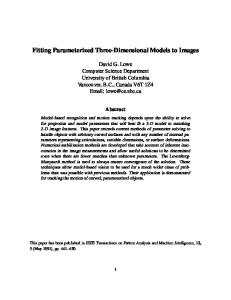
u1 u2 u3 v 00 u1 u2 u3 v0

Tv0 v0 w40

w30

→ w20

w1 w2 w3 w4

w1 w2 w3 w4

Fig. 1. Construction of the “tree structure” for a vertex v 0 ∈ V2 .

deleting the arc (wj , v) in I 0 is easy to see. Thus the modified instance is so far equivalent to I. Notice also that the vertices in I 00 that have degree larger than three are exactly the degree-four vertices in V2 . In order to decrease the degree of these vertices, we carry out the following modifications. For each vertex v 0 ∈ V2 , with N + (v 0 ) = {u1 , u2 , u3 }, remove (v 0 , u1 ) and (v 0 , u2 ), add a new vertex v 00 , and insert the three arcs (v 0 , v 00 ), (v 00 , u1 ), and (v 00 , u2 ) (see Figure 1). This concludes the construction of I 00 and we now prove the correctness. Let Tv0 be the subgraph induced by {v 0 , v 00 , u1 , u2 , u3 } where v 0 ∈ V2 . It is enough to show that exactly two arcs from Tv0 have to be removed in such a way that there remains only one path from v 0 to exactly one of the ui . Indeed, we have to remove at least two arcs: otherwise, two sinks will belong to the same connected component. Next, due to Lemma 1, it is not possible to remove more than two arcs from Tv0 . Moreover, using again Lemma 1, the two discarded arcs leave a single path from v 0 to exactly one of the ui . This completes the proof. t u

4

Parameterized Complexity: Bounded Solution Size

In this section, we investigate the influence of the parameter solution size k on the complexity of DAG Partitioning. To this end, notice that in Lemma 1 we proved that any minimal solution does not create new sinks. Hence, the task is to separate at minimum cost the existing sinks by deleting arcs without creating new ones. Note that this is very similar to the Multiway Cut problem: In Multiway Cut the task is to separate at minimum cost the given terminals. Multiway Cut was shown by Xiao [8] to be solvable in O(2k min(n2/3 , m1/2 )nm) time. However, the algorithm relies on minimum cuts and is rather complicated. In contrast, by giving a simple search tree algorithm running in O(2k · n2 ) time for DAG Partitioning, we show that the additional constraint to not create new sinks makes the problem arguably simpler. Our search tree algorithm exploits the fact that no new sinks are created in the following way: Assume that there is a vertex v with only one outgoing arc pointing to a vertex u. Then, for any minimal solution, u and v are in the same connected component. This leads to the following data reduction rule, which enables us to provide the search tree algorithm. It is illustrated in Figure 2.

100 0

a

a

1

1

b

c

100 1

2 d

2

100 100 b0

c0

a

100 Rule 1 applied to c

−−−−−−−−−−−−→

0

a

b 1

100

100

1 b0

1 d

4

c0

Fig. 2. Exemplary DAG Partitioning instance. Reduction Rule 1 transforms the instance into an equivalent instance: All paths from any vertex to c0 can be disconnected with the same costs as before. In every solution with costs less than 100, a must be in the same component as a0 and b must be in the same component as b0 . Let S = {a0 , b0 , c0 } be the sinks. Furthermore, d is a sink in D[V \ S] which must be disconnected from all but one sink. However, since a is adjacent to d removing the cheapest arc (d, a0 ) does not lead to a solution, because a0 and c0 would remain in the same component. In contrast, by removing (a, c0 ), (b, c0 ) and (d, c0 ) one obtains the unique solution, which has cost 6.

Reduction Rule 1 Let v ∈ V be a vertex with outdegree one and u its unique out-neighbor. Then for each arc (w, v) ∈ A, add an arc (w, u) with the same weight. If there already is an arc (w, u) in A, then increase the weight of (w, u) by ω(w, v). Finally, delete v. The correctness of this rule follows from the discussion above. Clearly, to a vertex v ∈ V , it can be applied in O(n) time. Thus, in O(n2 ) time, the input graph can be reduced until no further reduction by Reduction Rule 1 is possible. Thereafter, each vertex has at least two outgoing arcs and, thus, there is a vertex that has at least two sinks as out-neighbors. Exactly this fact we exploit for a search tree algorithm, yielding the following theorem: Theorem 3. DAG Partitioning can be solved in O(2k · n2 ) time. Proof. Since each connected component can be treated independently, we assume without loss of generality that the input graph D is connected. Moreover, we assume that Reduction Rule 1 is not applicable to D. Let S be the set of sinks in D. If all vertices are sinks, then D has only one vertex and we are done. Otherwise, let r be a sink in D[V \ S] (such a sink exists, since any subgraph of an acyclic graph is acyclic). Then the d arcs going out of r all end in sinks, that is, r is directly connected to d sinks. Since Reduction Rule 1 is not applicable, d > 1, and at most one of the d arcs may remain. We recursively branch into d cases, each corresponding to the deletion of d − 1 arcs. In each branch, k is decreased by d − 1 and the recursion stops as soon as it reaches 0. Thus, we have a branching vector (see e. g. [7]) of (d − 1, d − 1, . . . , d − 1), which | {z } d

yields a branching number not worse than 2, since 2d−1 ≥ d for every d ≥ 2. Therefore, the size of the search tree is bounded by O(2k ). Fully executing Reduction Rule 1 and finding r can all be done in O(n2 ) time. t u Limits of Kernelization and Parameterized Algorithms. In the remainder of this section we investigate the theoretical limits of kernelization and

parameterized algorithms with respect to the parameter k. Specifically, we show that unless the exponential time hypothesis (ETH) fails, DAG Partitioning cannot be solved in subexponential time, that is, the running time stated in Theorem 3 cannot be improved to 2o(k) poly(n). Moreover, by applying a framework developed by Bodlaender et al. [2] we prove that DAG Partitioning, unless NP ⊆ coNP/poly, does not admit a polynomial kernel with respect to k. Towards both results, we first recall the Karp reduction (a polynomial-time computable many-to-one reduction) from 3-SAT into DAG Partitioning given by Alamdari and Mehrabian [1]. The 3-SAT problem is, given a formula F in conjunctive normal form with at most three literals per clause, to decide whether F admits a satisfying assignment. Lemma 2 ([1, Sect. 2]). There is a Karp reduction from 3-SAT to DAG Partitioning. Proof. We briefly recall the construction given by Alamdari and Mehrabian [1]. Let ϕ be an instance of 3-SAT with the variables x1 , . . . , xn and the clauses C1 , . . . Cm . We construct an instance (D, ω, k) with k := 4n + 2m for DAG Partitioning that is a yes-instance if and only if ϕ is satisfiable. Therein, the weight function ω will assign only two different weights to the arcs: A normal arc has weight one and a heavy arc has weight k + 1 and thus cannot be contained in any solution. Construction: We start constructing the DAG D by adding the special vertices f, f 0 , t and t0 together with the heavy arcs (f, f 0 ) and (t, t0 ). The vertices f 0 and t0 will be the only sinks in D. For each variable xi , introduce the vertices xti , xfi , xi and xi together with the heavy arcs (t, xti ) and (f, xfi ) and the normal arcs (xti , xi ), (xti , xi ), (xfi , xi ), (xfi , xi ), (xi , f 0 ), (xi , f 0 ), (xi , t0 ), and (xi , t0 ). For each clause C, add a vertex C together with the arc (t0 , C). Finally, for each clause C and each variable xi , if the positive (or negative) literal of xi appears in C, then add the arc (C, xi ) ((C, xi ), resp.). This completes the construction of D. Correctness: One can prove that (D, ω, k) is a yes-instance for DAG Partitioning if and only if ϕ is satisfiable. Limits of Parameterized Algorithms. The Exponential Time Hypothesis (ETH) was introduced by Impagliazzo et al. [5] and states that 3-SAT cannot be solved in 2o(n) poly(n) time, where n denotes the number of variables. Corollary 1. Unless the ETH fails, DAG Partitioning cannot be solved in 2o(k) poly(n) time. Proof. The reduction provided in the proof of Lemma 2 reduces an instance of 3-SAT consisting of a formula with n variables to an equivalent instance (D, ω, k) of DAG Partitioning with k = 4n + 2m. In order to prove Corollary 1, it remains to show that we can upper-bound k by a linear function in n. Fortunately, this is done by the so-called Sparsification Lemma [5], which allows us to assume that the number of clauses in the 3-SAT instance that we reduce from is linearly bounded in the number of variables. t u

Limits of Problem Kernelization. We first recall the basic concepts and the main theorem of the framework introduced by Bodlaender et al. [2]. Theorem 4 ([2, Corollary 10]). If some set L ⊆ Σ ∗ is NP-hard under Karp reductions and L cross-composes into the parameterized problem Q ⊆ Σ ∗ × N, then there is no polynomial-size kernel for Q unless NP ⊆ coNP/poly. Here, a problem L cross-composes into a parameterized problem Q if there is a polynomial-time algorithm that transform the instances I1 , . . . , Is of Q into an instance (I, k) for L such that k is bounded by a polynomial in maxsi=1 |Ij | + log s and (I, k) ∈ L if and only if there is an instance Ij ∈ Q, where 1 ≤ j ≤ s. Furthermore, it is allowed to assume that the input instances I1 , . . . , Is belong to the same equivalence class of a polynomial equivalence relation R ⊆ Σ ∗ × Σ ∗ , that is, an equivalence relation such that it can be decided in polynomial time whether two inputs are equivalent and each set S ⊆ Σ ∗ is partitioned into at most maxx∈S (|x|)O(1) equivalence classes. In the following we show that 3-SAT cross-composes into DAG Partitioning parameterized by k. In particular, we show how the reduction introduced in Lemma 2 can be extended to a cross-composition. Lemma 3. 3-SAT cross-composes to DAG Partitioning parameterized by k. Proof. Let ϕ1 , . . . , ϕs be instances of 3-SAT. We assume that each of them has n variables and m clauses. This is obviously a polynomial equivalence relation. Moreover, we assume that s is a power of two, as otherwise we can take multiple copies of one of the instances. We construct a DAG D = (V, A) that forms together with an arc-weight function ω and k := 4n + 2m + 4 log s an instance of DAG Partitioning that is a yes-instance if and only if ϕi is satisfiable for at least one 1 ≤ i ≤ s. Construction: For each instance ϕi let Di be the DAG constructed as in the proof of Lemma 2. Note that (Di , k 0 ) with k 0 := 4n + 2m is a yes-instance if and only if ϕi is satisfiable. To distinguish them between multiple instances, we denote the special vertices f, f 0 , t, and t0 in Di by fi , fi0 , ti , and t0i . For all 1 ≤ i ≤ s, we add Di to D and we identify the vertices f1 , f2 , . . . , ft to a vertex f and, analogously, we identify the vertices f10 , f20 , . . . , ft0 to a vertex f 0 . Furthermore, we add the vertices t, t0 , and t00 together with the heavy arcs (t, t00 ) and (t, t0 ) to D. As in the proof of Lemma 2, a heavy arc has weight k + 1 and thus cannot be contained in any solution. All other arcs, called normal, have weight one. Add a balanced binary tree O with root in t00 and the leaves t1 , . . . , ts formed by normal arcs which are directed from the root to the leaves. For each vertex in O, except for t00 , add a normal arc from f . Moreover, add a balanced binary tree I with root t0 and the leaves t01 , . . . , t0s formed by normal arcs that are directed from the leaves to the root. For each vertex in I, except for t0 , add a normal arc to f 0 . This completes the construction of D. Correctness: One can prove that (D, ω, k) is a yes-instance if and only if ϕi is satisfiable for at least one 1 ≤ i ≤ s. t u Lemma 3 and Theorem 4 therefore yield:

Theorem 5. DAG Partitioning does not have a polynomial-size kernel with respect to k, unless NP ⊆ coNP/poly. We note that Theorem 5 can be strengthened to graphs of constant diameter or unweighted graphs.

5

Partitioning DAGs of Bounded Treewidth

In the meme tracking application, edges always go from longer to shorter phrases by omitting or modifying words. It is thus plausible that the number of phrases of some length on a path between two phrases is bounded. Thus, the underlying graphs are tree-like and in particular have bounded treewidth. In this section, we investigate the computational complexity of DAG Partitioning measured in terms of distance to “tree-like” graphs. Specifically, we show that if the input graph is indeed a tree with uniform edge weights, then we can solve the instance in linear time by data reduction rules (see Theorem 6). Afterwards, we prove that this can be extended to weighted graphs of constant treewidth and, actually, we show that DAG Partitioning is fixed-parameter tractable with respect to treewidth. This improves the algorithm for pathwidth given by Alamdari and Mehrabian [1], as the treewidth of a graph is at most its pathwidth. Warm-Up: Partitioning Trees Theorem 6. DAG Partitioning is solvable in linear time if the underlying undirected graph is a tree with uniform edge weights. To prove Theorem 6, we employ data reduction on the tree’s leaves. Note that Reduction Rule 1 removes all leaves of a tree that have outdegree one and leaves that are the only out-neighbor of their parent. In this case, Reduction Rule 1 can be realized by merely deleting such leaves. In cases where Reduction Rule 1 is not applicable to any leaves, we apply the following data reduction rule: Reduction Rule 2 Let v ∈ V be a leaf with in-degree one and in-neighbor w. If w has more than one out-neighbor, then delete v and decrement k by one. We can now prove that as long as the tree has leaves, one of Reduction Rule 1 and Reduction Rule 2 applies, thus proving Theorem 6. Partitioning DAGs of Bounded Treewidth. We note without proof that DAG Partitioning can be characterized in terms of monadic second-order logic (MSO), hence it is FPT with respect to treewidth (see e. g. [7]). However, the running time bound that this approach yields is far from practical. Therefore, we give an explicit dynamic programming algorithm. Theorem 7. Given a tree decomposition of the underlying undirected graph of 2 width w, DAG Partitioning can be solved in O(2O(w ) · n) time. Hence, it is fixed-parameter tractable with respect to treewidth.

Suppose we are given D = (V, A), ω, k and a tree decomposition (T, β) for the underlying undirected graph of D of width w. Namely, T is a tree and β is a mapping that assigns to every node x in V (T ) a set Vx = β(x) ⊆ V called a bag (for more details on treewidth see e. g. [7]). We assume without loss of generality, that the given tree decomposition is nice and is rooted in a vertex r with an empty bag. For a node x of V (T ), we denote by Ux the union of Vy over all y descendant of x, AVx denotes A(D[Vx ]), and AU x denotes A(D[Ux ]). Furthermore, for a DAG G we define the transitive closure with respect to the reachability as Reach∗ (G) := (V (G), A(G) ∪ {(u, v) | u, v ∈ V (G), u 6= v, and there is an oriented path from u to v in G}). Solution Patterns. Our algorithm is based on leaf to root dynamic programming. The behavior of a partial solution is described by a structure which we call a pattern. Let x be a node of T and Vx its bag. Let P be a DAG with V (P ) consisting of Vx and at most |Vx | additional vertices such that each vertex in V (P ) \ Vx is a non-isolated sink. Let Q be a partition of V (P ) into at most |Vx | sets Q1 , . . . , Qq , such that each connected component of P is within one set of Q and each Qi contains at most one vertex of V (P ) \ Vx . Let R be a subgraph of P [Vx ]. We call (P, Q, R) a pattern for x. In the next paragraphs, we give an account of how the pattern (P, Q, R) describes a partial solution. Intuitively, the DAG P stores the vertices of a bag and the sinks these vertices can reach in the graph modified by the partial solution. The partition Q refers to a possible partition of the vertices of the graph such that each part is a connected component and each connected component contains exactly one sink. Finally, the graph R is the intersection of the partial solution with Vx . Formally, a pattern describes a partial solution as follows. Let A0 ⊆ AU x be a set of arcs such that no connected component of Dx (A0 ) = D[Ux ] \ A0 contains two different sinks in Ux \ Vx and every sink in a connected component of Dx (A0 ) which contains a vertex of Vx can be reached from some vertex of Vx in Dx (A0 ). A sink in Ux \ Vx is called interesting in Dx (A0 ) if it is reachable from at least one vertex of Vx . Let Px (A0 ) be the DAG on Vx ∪ V 0 , where V 0 is the set of interesting sinks in Dx (A0 ) such that there is an arc (u, v) in Px (A0 ) if the vertex u can reach the vertex v in the DAG Dx (A0 ). Let Qx (A0 ) be the partition of Vx ∪ V 0 such that the vertices u and v are in the same set of Qx (A0 ) if and only if they are in the same connected component of Dx (A0 ). Finally, by Rx (A0 ) we denote the DAG D[Vx ] \ A0 . Let (P, Q, R) be a pattern for x. We say that A0 satisfies the pattern (P, Q, R) at x if no connected component of Dx (A0 ) contains two different sinks in Ux \ Vx , every sink in a connected component of Dx (A0 ) which contains a vertex of Vx can be reached from some vertex of Vx in Dx (A0 ), P = Px (A0 ) (there is an isomorphism between P and Px (A0 ) which is identical on Vx , to be precise), Q is a coarsening of Qx (A0 ), and R = Rx (A0 ). Formally, Q is a coarsening of Qx (A0 ) if for each set Q ∈ Qx (A0 ) there exists a set Q0 ∈ Q such that Q ⊆ Q0 . Note, that some coarsenings of Qx (A0 ) may not form a valid pattern together with Px (A0 ) and Rx (A0 ).

For each node x of V (T ) we have a single table Tabx indexed by all possible patterns for x. The entry Tabx (P, Q, R) stores the minimum weight of a set A0 that satisfies the pattern (P, Q, R) at x. If no set satisfies the pattern, we store ∞. As the root has an empty bag, Tabr has exactly one entry containing the minimum weight of set A0 such that in Dr (A0 ) = D \ A0 no connected component contains two sinks. Obviously, such a set forms a solution for D. Hence, once the tables are correctly filled, to decide the instance (D, ω, k), it is enough to test whether the only entry of Tabr is at most k. The Algorithm. Now we show how to fill the tables. First we initialize all the tables by ∞. By updating the entry Tabx (P, Q, R) with m we mean setting Tabx (P, Q, R) := m if m < Tabx (P, Q, R). For a leaf node x we try all possible V 0 subsets A0 ⊆ AU x = Ax , and for each of them and for each coarsening Q of Qx (A ) 0 0 0 we update Tabx (Px (A ), Q, Rx (A )) with ω(A ). Note that in this case, as there are no vertices in Px (A0 ) \ Vx , every coarsening of Qx (A0 ) forms a valid pattern together with Px (A0 ) and Rx (A0 ). In the following we assume that by the time we start the computation for a certain node of T , the computations for all its children are already finished. Consider now the case, where x is a forget node with a child y, and assume that v ∈ Vy \ Vx . For each pattern (P, Q, R) for y we distinguish several cases. In each of them we set R0 = R \ {v}. If v is isolated in P and there is a set {v} in Q (case (i)), then we let P 0 = P \ {v}, Q0 be a partition of V (P 0 ) obtained from Q by removing the set {v}, and update Tabx (P 0 , Q0 , R0 ) with Taby (P, Q, R). If v is a non-isolated sink and v ∈ Qi ∈ Q such that Qi ⊆ Vy (case (ii)), then we update Tabx (P, Q, R0 ) with Taby (P, Q, R) (P 0 = P, Q0 = Q in this case). If v is not a sink in P and there is no sink in V (P )\Vy such that v is its only in-neighbor (case (iii)), then let P 0 = P \ {v} and Q0 be a partition of V (P 0 ), obtained from Q by removing v from the set it is in, and update Tabx (P 0 , Q0 , R0 ) with Taby (P, Q, R). If there is a sink u ∈ V (P ) \ Vy such that v is its only in-neighbor and {u, v} is a set of Q (case (iv)), then let P 0 = P \ {u, v} and Q0 be a partition of V (P 0 ), obtained from Q by removing the set {u, v}, and update Tabx (P 0 , Q0 , R0 ) with Taby (P, Q, R). We don’t do anything for the patterns (P, Q, R) which do not satisfy any of the above conditions. Next, consider the case, where x is an introduce node with a child y, and assume that v ∈ Vx \ Vy and B is the set of arcs of AVx incident to v. For each B 0 ⊆ B and for each pattern (P, Q, R) for y such that there is a Qi in Q with NB 0 (v) ⊆ Qi we let R0 = (Vx , A(R)∪B 0 ), D0 = (V (P )∪{v}, A(P )∪B 0 ), P 0 = Reach∗ (D0 ) and we distinguish two cases. If B 0 = ∅, then for every Qi ∈ Q we let Q0 be obtained from Q by adding v to the set Qi and update Tabx (P 0 , Q0 , R0 ) with Taby (P, Q, R) + ω(B). Additionally, for Q0 obtained from Q by adding the set {v} we also update Tabx (P 0 , Q0 , R0 ) with Taby (P, Q, R) + ω(B). If B 0 is non-empty, then let Qi be the set of Q with NB 0 (v) ⊆ Qi and let Q0 be obtained from Q by adding v to the set Qi . We update Tabx (P 0 , Q0 , R0 ) with Taby (P, Q, R) + ω(B) − ω(B 0 ). Finally, consider the case that x is a join node with children y and z. For each pair of patterns (Py , Qy , R) for y and (Pz , Qz , R) for z such that Qy and Qz

partition the vertices of Vy = Vz = Vx in the same way we do the following. Let D0 be the DAG obtained from the disjoint union of Py and Pz by identifying the vertices in Vx and P 0 = Reach∗ (D0 ). Let Q0 be a partition of V (P 0 ) such that it partitions Vx in the same way as Qy and Qz and for each u ∈ V (P 0 ) \ Vx add u to a set Qi which contain a vertex v with (v, u) being an arc of P 0 . It is not hard to see, that there is always exactly one such set Qi , as there are no arcs between different sets in Py and Pz . If some set Q ∈ Q0 contains more than one vertex of V (P 0 )\Vx , then continue with a different pair of patterns. Otherwise, we update Tabx (P 0 , Q0 , R) with Taby (Py , Qy , R) + Tabz (Pz , Qz , R) − ω(AVx ) + ω(A(R)).

6

Outlook

We have presented two parameterized algorithms for DAG Partitioning, one with parameter solution size k and one with parameter treewidth w. In particular the algorithm for the parameter k seems suitable for implementation; in combination with data reduction, this might allow to solve optimally instances for which so far only heuristics are employed [6]. On the theoretical side, one open question is whether we can use the Strong Exponential Time Hypothesis (SETH) to show that there is no O((2−ε)k poly(n)) time algorithm for DAG Partitioning. Another question is whether there is an algorithm solving the problem in O(2O(w log w) · n) or even O(2O(w) · n) time, where 2 w is the treewidth, as the O(2O(w ) · n) running time of our algorithm still seems to limit its practical relevance.

References [1] S. Alamdari and A. Mehrabian. On a DAG partitioning problem. In Proc. 9th WAW, volume 7323 of LNCS, pages 17–28. Springer, 2012. [2] H. L. Bodlaender, B. M. P. Jansen, and S. Kratsch. Cross-composition: A new technique for kernelization lower bounds. In Proc. 28th STACS, volume 9 of LIPIcs, pages 165–176. Dagstuhl Publishing, 2011. [3] E. Dahlhaus, D. S. Johnson, C. H. Papadimitriou, P. D. Seymour, and M. Yannakakis. The complexity of multiterminal cuts. SIAM J. Comput., 23 (4):864–894, 1994. [4] R. G. Downey and M. R. Fellows. Parameterized Complexity. Springer, 1999. [5] R. Impagliazzo, R. Paturi, and F. Zane. Which problems have strongly exponential complexity? J. Comput. System Sci., 63(4):512–530, 2001. [6] J. Leskovec, L. Backstrom, and J. M. Kleinberg. Meme-tracking and the dynamics of the news cycle. In Proc. 15th ACM SIGKDD, pages 497–506. ACM, 2009. [7] R. Niedermeier. Invitation to Fixed-Parameter Algorithms. Oxford University Press, 2006. [8] M. Xiao. Simple and improved parameterized algorithms for multiterminal cuts. Theory Comput. Syst., 46:723–736, 2010.