On Wireless Social Community Networks Mohammad Hossein Manshaei∗ , Julien Freudiger∗ , Mark F´elegyh´azi∗ , Peter Marbach† , and Jean-Pierre Hubaux∗ ∗
Laboratory for computer Communications and Applications (LCA), EPFL, Lausanne, Switzerland Email:{hossein.manshaei, julien.freudiger, mark.felegyhazi, jean-pierre.hubaux}@epfl.ch † Department of Computer Science, University of Toronto, Canada Email:
[email protected]
Abstract—Wireless social community networks are emerging as a new alternative to provide wireless data access in urban areas. By relying on users in the network deployment, a wireless community can rapidly deploy a high-quality data access infrastructure in an inexpensive way. But, the coverage of such a network is limited by the set of access points deployed by the users. Currently, it is not clear if this paradigm can serve as a replacement of existing centralized networks operating in licensed bands (such as cellular networks) or if it should be considered as a complimentary service only. This question currently concerns many wireless network operators. In this paper, we study the dynamics of wireless social community networks using a simple analytical model. In this model, users choose their service provider based on the subscription fee and the offered coverage. We show that the evolution of social community networks depends on their initial coverage, the subscription fee, and the user preferences for coverage. We conclude that by using an efficient static or dynamic pricing strategy, the wireless social community can obtain a high coverage. Using a game-theoretic approach, we then study a case where the mobile users can choose between the services provided by a licensed band operator and those of a social community. We show that for specific distribution of user preferences, there exists a Nash Equilibrium for this non-cooperative game. Finally, we study the cooperative scenario where both infrastructures belong to one operator.
I. I NTRODUCTION Wireless networks have traditionally been deployed and operated by central authorities. The centralized management of wireless network infrastructures guarantees a high quality of service (QoS) in terms of network coverage, but at the expense of substantial deployment and maintenance costs. Having users form wireless social communities, a wireless network operator can share infrastructure costs with its customers. The WiFi technology (i.e., IEEE 802.11 devices) is a viable option: WiFi networks offer an inexpensive high-speed wireless access to users and do not necessitate expensive investments because the technology operates in an unlicensed frequency band. Thus, there is no need for the operator to make substantial initial investment to buy the spectrum license. Furthermore, the access points (AP) are inexpensive, easy to deploy and maintain. Still, the wireless social community typically has a limited coverage, which depends on the size of the network. Wireless social community networks could be at the core of the next wireless generation. In this paper, we are concerned with the potential of wireless social communities to compete with traditional licensed band networks. We first evaluate the evolution of wireless social community networks by modeling users’ payoffs as a function
of the subscription fee1 , as well as the operators’ provided coverage. We discuss static and dynamic strategies for attracting new subscribers to improve the coverage of social community networks. To the best of our knowledge, this is the first model to address and evaluate the strategies of social community operators, taking into account the preferences of users in term of coverage and subscription fees. Then, we discuss the competition between social community operators and traditional licensed band operators using a game-theoretic approach. We investigate the strategies of the operators in a competition and the corresponding outcomes of the game. In the hope of mutually beneficial results, we identify a Nash Equilibrium in this game and discuss the possible cooperation between the operators. We believe that our paper gives an insight to understanding the evolution of wireless social communities in the presence of traditional wireless access providers. The paper is organized as follows. In Section II, we characterize the properties of users, the licensed band operator and the social community operator. In Section III, we present the main results and contributions of this paper. In Section IV and V, we evaluate the dynamics of these networks separately and derive the maximum payoff and the corresponding optimal number of subscribers. In Section VI, we model the competition of these two types of network operators and discuss their coexistence. In Section VII, we discuss the cooperative scenario where both infrastructures belong to one operator. Finally, in Section VIII and IX we discuss the related work and some open questions. II. S YSTEM M ODEL We consider a network service area, where users have the choice between the services offered by two wireless network operators. We assume that one operator deploys his own network infrastructure in a licensed band (e.g., WiMAX) to provide wireless access to users. The other operator relies on technologies operating in unlicensed bands (e.g., WiFi) and involves the wireless APs operated by the users to establish a wireless social community. Consequently, we refer to the two operators as the licensed band operator (LBO) and the social community operator (SCO). Let Qi ∈ [0, 1] be the coverage provided by a given network operator i. We assume that the users evaluate the 1 Note that the subscription fee corresponds to the price users have to pay. Hence, we use the two terms interchangeably in the paper.
2
usefulness of the social community network based on the provided coverage and subscription fee. The study of more sophisticated user preferences is part of our future work (as discussed in Section IX). Next, we characterize the behavior of the users as well as the two operators by defining their appropriate payoff functions. A. Mobile Users We assume that N users, distributed in the service area of the service providers, are potentially interested in wireless access. They subscribe to a wireless network operator based on their coverage requirements and the subscription fees. Assume that user v subscribed to operator i ∈ {LBO, SCO}. Then, we model the payoff of user v as a function of the coverage provided by network operator i (Qi ), the subscription fee of operator i (Pi ), and a user type parameter av that characterizes its subscription preference. For any user v the payoff under operator i is: uiv = av · Qi − Pi . A user v subscribes to an operator if its payoff using that operator is greater than zero, i.e., uiv > 0. The user type av for user v defines the coverage requirements of user v. Users with high av subscribe to operator i even if it has a low coverage Qi and high subscription fee Pi . On the contrary, users with low av require high Qi and low Pi . A fraction of users with very small av will refrain from subscribing to any operator, because they are not satisfied with the available coverage and subscription fees. Note that we consider a payoff function uv that depends linearly on the available coverage. We discuss the extension of the model to generic concave payoff functions in Section IX. For simplicity, let us assume that av is a random variable uniformly distributed in [α, β] as shown in Fig. 1(a) and that this distribution is known to the operators. We further assume that users reconsider their subscriptions periodically (e.g., beginning of the month) and they are able to change it if they have another option. A mobile user v switches from operator i to operator j if and only if ujv > uiv > 0. We assume that there is no cost of changing operators. B. Licensed Band Operator (LBO) LBOs obtain a spectrum license to use a given frequency spectrum. They typically use a collision free protocol (e.g., WiMAX) to provide the wireless services. We suppose that the LBO has full coverage (i.e., Q` = 1) and a subscription fee P` . We denote the payoff of the LBO at time t by u` [t]. This payoff is a function of the fraction of users who subscribed to the LBO 0 ≤ n` [t] ≤ 1 (i.e., n` [t] = 1 means that all N mobile users have subscribed in the LBO) and the cost c` of the LBO infrastructure (e.g., to deploy and maintain base stations, to acquire the spectrum licenses, etc.). We define the payoff of the LBO at time t as: u` [t] =
N · n` [t] · P` − c` ,
(1)
where P` is the price charged by the LBO to each user and c` is the infrastructure cost for the LBO.
C. Social Community Operator (SCO) Subscribers to the SCO participate in the deployment of the network in the unlicensed band (e.g., by sharing their IEEE 802.11 APs). We assume that the users pay a monthly subscription fee Ps to the SCO to be a member of the community. This subscription fee is most likely to be substantially smaller than the LBO subscription fee P` . We assume that for this price, the SCO provides the APs to the users and maintains the network infrastructure (e.g., the software that enables social community services). Thus, the SCO has a small cost cs for deploying the service. We assume that SCOs previously agreed with ISPs to let users share their APs. We discuss the strategic service agreements between ISPs and SCOs [2] in Section IX. The coverage Qs of the social network, unlike for the LBO, depends on the number of users who decide to join the SCO’s network. We assume that Qs is a linear function of the fraction of users who subscribed in the SCO, 0 ≤ ns [t] ≤ 1, as shown in Fig. 1(b), i.e., Qs [t] = ns [t]. We also assume that the best coverage (i.e., Qs = 1) is obtained if and only if all users subscribe to the community. With this coverage function, we assume a channel assignment scheme as introduced in [7], i.e., a non-interfering channel assignment obtained via local channel bargaining. The payoff function of the SCO at time t is then: us [t] = N · ns [t] · Ps − cs ,
(2)
where Ps is the price paid by the user who subscribe to the social community and cs is the infrastructure cost of the SCO. f(av)
Qs 1
1/(β−α)
Qs[t]
α
Ps /Q
(a)
Pl
β
av
ns[t]
1
ns
(b)
Fig. 1. System model: (a) Uniform distribution of user types. (b) Relation between subscribers and the social community coverage at time t.
III. M AIN R ESULTS AND C ONTRIBUTIONS The model presented in the precedent section is evaluated in two scenarios: (1) a monopoly, in which a unique operator offers the wireless access, and (2) a duopoly, in which both operators compete for subscribers. In the rest of the paper, we obtain the pricing strategies that maximizes the payoff of the operators in both settings. We first show that the strategy maximizing the LBO revenue in a monopoly depends on the spread of the distribution of user types. When users are widely distributed (β > 2α), the LBO maximizes its payoff by behaving selfishly. In other terms, the LBO sets a high subscription fee such that only users with a high user type av subscribe. In the case of a narrow distribution of user types (β ≤ 2α), the LBO should set a subscription fee
3
such that all users subscribe to its service. The payoff achieved with the wide distribution is higher than that achieved with the narrow distribution. Next, we analyze the dynamics of the SCO in a monopoly; we consider two pricing strategies: static and dynamic pricing. In the static pricing strategy, the subscription fee is not changed during the evolution of the social community. In the dynamic pricing strategy, the coverage Qs of the social community directly affects the subscription fee. We derive the potential convergence of the SCO coverage for both pricing strategies and determine the price which achieves the maximal SCO payoff. We observe that the SCO payoff in monopoly is not only affected by the distribution of user types, but also by its initial coverage Qs [0]. We conclude that the SCO should first bootstrap its network with low prices to reach a fair coverage before adjusting its price to maximize its revenue. This conclusion nicely matches the behavior of real wireless social communities [3]. Finally, if the distribution of user types is narrow, then the SCO coverage potentially converges to 1 whereas for a wide user type distribution, it is less than 1. However, the achieved payoff is larger for the wide user type distribution. We finally consider the co-existence of a LBO and a SCO and compute their respective best responses. The competition ends up in two scenarios depending again on the distribution of user types: (1) if β ≥ 32 α, then there is a Nash Equilibrium in which both operators have subscribers, else (2) if β < 32 α, then there is no social community coverage with which the calculated Nash Equilibrium is satisfied. A Nash Equilibrium strategy profile results in lower subscription fees and more subscribers. Because it forces the operators to have an aggressive pricing strategy, competition benefits mobile users. We finally show that wireless operators do not have an economic incentive to deploy both a social community and a licensed band wireless access. IV. R EVENUE A NALYSIS OF A L ICENSED BAND O PERATOR First, we assume that only the LBO provides wireless data access in the service area. We derive the final fraction of users n` who subscribe to the LBO. For uniform distribution of user types, we obtain the following: n`
= = =
P r{av − P` > 0} P r{max{α, P` } < av < β} 1 (β − max{α, P` }) β−α
(3)
As the cost c` of operating the LBO network is fixed, and n` is determined by the user types av and the price P` , the LBO optimizes its payoff u` expressed in (1) by properly choosing P` . At this point, we emphasize that the solutions for the optimal prices and payoffs depend on the distribution of user types defined by the parameters α and β. Accordingly, we distinguish two cases throughout our paper: (i) narrow distribution of user types meaning that β ≤ 2α, and (ii) wide distribution of user types meaning that β > 2α. We present the solutions of the optimization problem for the LBO below.
A. Narrow Distribution of User Types Recall the assumption that β ≤ 2α. To find the optimal payoff for the LBO, let us substitute (3) into (1): u` =
N (β − max{α, P` }) · P` − c` β−α
(4)
Taking the derivative of (4) with respect to P` and imposing it equal to 0, we obtain the optimal subscription fee that maximizes the LBO’s payoff: β } (5) 2 For β ≤ 2α, the optimal price is α and the optimal payoff for the LBO is uopt = N α − c` . The corresponding fraction ` of subscribed users is then nopt = 1. ` P`opt = max{α,
B. Wide Distribution of User Types The solution changes if we consider a wide distribution of user types, i.e. β > 2α. Then, the optimal price in (5) is: P`opt =
β 2
(6)
The corresponding optimal payoff can be written as uopt = ` 2 · β4 − c` . Finally, the the maximum fraction of users nopt ` who subscribe to LBO is: β 1 nopt (7) = · ` 2 β−α N β−α
Note that the maximum payoff depends on the distribution of user types [α, β]. Equation (7) also shows that the LBO acts selfishly by ignoring a subset of its potential users (up to half of the users), in order to maximize its payoff. We observe that the optimal payoff of the LBO for a wide distribution of user types is always larger than that of narrow distribution. V. DYNAMICS OF A S OCIAL C OMMUNITY O PERATOR In this section, we assume that the SCO is the only wireless access provider. We study the evolution of the SCO’s network. Recall the assumption that the user types are uniformly distributed in [α, β]. Let Qs [0] be the initial coverage (i.e., the number of users who initially subscribe to the service). Note that Qs [0] > 0, otherwise the social community never forms. User v will subscribe to the wireless service at time t if and only if usv is strictly greater than zero for a given coverage Qs [t]: usv = av · Qs [t] − Ps > 0 (8) We compute the coverage achieved by the SCO at time t as follows: Qs [t] = = = =
ns [t] P r{av Qs [t − 1] − Ps > 0} s P r{max{α, QsP[t−1] } < av < β} 1 β−α (β
s − max{α, QsP[t−1] })
(9)
In Section V-A and V-B, we assume that the SCO applies a static pricing strategy and does not adapt its price to the actual coverage value in the network. Assume for example that the
4
coverage value Qs [t] is evaluated each month. It is reasonable to assume that the SCO keeps its price fixed for a longer time period to preserve the clarity of pricing for the users. We study the benefits of dynamic pricing strategies in Section V-C.
Qs[0]
(a)
We derive the dynamics of the social community by looking at ∆Qs = Qs [t] − Qs [t − 1] (Equation (40) in Appendix A). As shown in Fig. 2, we observe that for a low price the social community reaches full coverage, whereas for a high price, it disappears. For a price Ps such that Qs,1 = Qs [0], the SCO final coverage is Qs [0]. Qs[0]
(a)
Q
0
1 Qs[0] Qs[0]
(b)
0
Qs,1
Q 1 Qs[0]
(c)
0
Q
1
Fig. 2. Dynamics of the SCO for a narrow distribution of user types: (a) Ps = 0, (b) 0 < Ps ≤ α, (c) Ps > α.
2) Wide Distribution of User Types: If the distribution of user types is such that β > 2α, we obtain an additional potential convergence point: p β + β 2 − 4(β − α)Ps Qs,2 = (11) 2(β − α) Hence, we have four potential convergence points Qs [∞] = {0, Qs,1 , Qs,2 , 1} (details given in part B of Appendix A). Because of Qs,2 , we can identify three more convergence scenarios shown in Fig. 3 (c) and (d). Note that Qs converges monotonically to Qs,2 as proved in Appendix B. B. Optimal Static Price In this subsection, we derive the optimal static price Psopt that maximizes the payoff of the SCO for various values of Qs [0], α and β. We assume that the SCO has an initial coverage Qs [0] > 0 and the number of subscribers to the social community evolves as a function of the price Ps .
1 Qs,2 Qs[0] Qs[0]
(b)
A. Convergence Points with a Static Pricing In the following analysis, we are interested in the potential convergence points Qs [∞], where the coverage (and hence the fraction of subscribed users) stabilizes. The convergence of the social community depends on the values of Ps , Qs [0], α, and β. As before, we obtain different solutions for various distributions of user types. 1) Narrow Distribution of User Types: If the user types are distributed such that β ≤ 2α, then we obtain three potential convergence points: Qs [∞] = {0, Qs,1 , 1} (details given in part A of Appendix A), where p β − β 2 − 4(β − α)Ps Qs,1 = (10) 2(β − α)
Q
Qs,1=0
0
Q 1Qs,2
Qs,1 Qs[0] Qs[0]
(c)
0
Qs[0] Qs,2
Qs,1 Qs[0]
(d)
0
Qs,1=Qs,2
1 Qs[0]
Q
1 Qs[0]
(e)
Q
Q
1
0
Fig. 3. Dynamics of SCO for a wide distribution of user types: (a) Ps = 0, β2 β2 (b) 0 < Ps ≤ α, (c) α < Ps < 4(β−α) , (d) Ps = 4(β−α) , (e) Ps > β2 . 4(β−α)
From the convergence scenarios presented in Section V-A, we observe that if the price selected by SCO is such that Qs,1 is bigger than the initial coverage Qs [0] (as shown in Fig. 2 (b) and Fig. 3 (b), (c) and (d)), then the SCO can never increase its coverage and consequently, the proportion of subscribers and its revenue. The reason is that in these cases the SCO’s coverage always converges to 0. According to the previously defined user type distributions, we consider two scenarios. 1) Narrow Distribution of User Types: For a narrow distribution of user types, the upper limit of the convergence is 1. Then, the SCO should select the price such that Qs,1 < Qs [0] (as illustrated in Fig. 2(b)). This means that: p β − β 2 − 4(β − α)Ps Qs,1 = = Qs [0] − ² (12) 2(β − α) where ² > 0 is a small positive value. From (12), we can express the value of Ps as, Ps = (Qs [0] − ²) · (β − (β − α) · (Qs [0] − ²)), and for ² → 0, Ps → Qs [0] · (β − (β − α) · Qs [0])
(13)
Note that the above price is always less than α for all Qs [0] ∈ [0, 1]. The final fraction of subscribed users is ns = 1 and the corresponding payoff is: us = N ·ns ·Ps −cs = N Qs [0]·(β −(β −α)·Qs [0])−cs (14) 2) Wide Distribution of User Types: Considering all convergence scenarios presented in Fig. 3, the SCO should select the price based on the initial coverage. For the optimal static price, the following scenarios can be distinguished: α : The results are the same as for the • If 0 < Qs [0] < β−α case where β ≤ 2α (see Appendix A for case (b) in Fig. 2 and 3). The optimal static price and payoff function can be calculated by Equation (13) and (14). α • If β−α < Qs [0] < 1: The fraction of subscribed users can either converge to 1 (Fig. 3(b)) or to Qs,2 (Fig. 3(c)). We provide the proof for the monotonic convergence to Qs,2 in
5
Appendix B. We have to compare these two cases to decide which one results in a superior payoff for the SCO for a given set of parameters. We assume that the SCO selects a static price such that the scenario corresponds to that of Fig. 3(c). Hence, the social community stabilizes in Qs,2 : us = =
N · Ps ·
N · Ps · Qs,2 − cs µ √ ¶ 2 β+
β −4(β−α)Ps 2(β−α)
(15) − cs
We then calculate Psopt that maximizes the SCO’s payoff function us by making the derivative of (15) with respect to Ps and imposing it equal to zero. β+ N Ps ∂us = −p +N ∂Ps β 2 − 4(β − α)Ps
p
β 2 − 4(β − α)Ps =0 2(β − α)
2 β2 9 (β − α)
(16)
For the price in (16), the following fraction of users subscribe to the SCO: 2 β = Qs = nopt (17) s 3β−α Finally, we have to take into account that the SCO does not decrease his price below the lower bound of QPss[t] , i.e., Ps P opt β = sopt = > α Qs [t] 3 ns
(18)
This means that the above optimal static price exists if and only if β > 3α. Accordingly, we have two subcases: − If 2α < β ≤ 3α, then the optimal price in (16) is smaller than α. One can show that the payoff function us = N · Ps · Qs,2 − cs is a concave function of Ps and it is decreasing in β2 the interval α < Ps < 4(β−α) . This results in the optimal price Psopt = α (i.e., Qs,2 = 1) and the maximum payoff value uopt = N α − cs . s − If β > 3α, then the solution in (16) defines the optimal static price. Consequently, the fraction of subscribed users is defined in (17). For these Psopt and nopt values, the optimal s β3 4 opt payoff of the SCO is us = N 27 (β−α)2 − cs . We have seen that the initial coverage Qs [0], and the distribution of user types determine the range of optimal static prices from which the SCO can select its price. In the next subsection, we assume that the SCO applies dynamic pricing strategies to better adapt the price Ps to the changing coverage. C. Dynamic Pricing Let us now assume that the SCO adjusts its price Ps at time t to follow the evolution of its network. The essential difference between static and dynamic pricing is that with dynamic pricing the SCO can maintain a lower price until a desired coverage is reached and then fine-tune the price. Since ∆Qs must be strictly positive, we derive the following condition on the dynamic price (details given in Appendix A): Ps [t] < −(β − α)Q2s [t − 1] + βQs [t − 1]
Ps [t] = −(β − α)Q2s [t − 1] + βQs [t − 1] − ²
(19)
(20)
where ² is a small positive value. Similar to the static price strategy, two main scenarios can be distinguished. 1) Narrow Distribution of User Types: Ps [t] is increasing in [0, 1] and its maximum value is α corresponding to Qs = 1. So the coverage of the SCO converges to 1 and us = N α−cs . 2) Wide Distribution of User Types: The maximum value β2 β of Ps [t] is 4(β−α) at Qs = 2(β−α) < 1. The SCO payoff is: us [t] = N ·
The optimal static price for this case is then: Psopt =
The right-hand side of (19) is always positive for all Qs ∈ [0, 1]. Thus, the SCO maintains the increase of the coverage by selecting appropriate dynamic prices Ps [t], such that,
1 Ps [t] (β − ) · Ps [t] − cs β−α Qs [t − 1]
(21)
Finally, we can express the SCO payoff as a function of Qs [t− 1] using Equation (20) when ² → 0: us [t] = N (β − α)(β − (β − α)Qs [t − 1])Q2s [t − 1] − cs (22) Using Equation (22), we can obtain the best price and covβ = 23 β−α erage that maximizes the SCO payoff, i.e., Qopt , s 2
3
β β 4 Psopt = 29 β−α , and uopt = 27 s (β−α)2 − cs . Considering the Ps lower bound on Qs [t] , we again conclude that the maximum value exists if β > 3α. If 2α < β < 3α, the best price is Psopt = α and coverage can potentially converge to 1.
VI. C OEXISTENCE OF A SCO AND A LBO So far, we evaluated the SCO and LBO individually and derived their optimal strategies in a monopoly. In this section, we consider a duopoly in which the simultaneous presence of the LBO and SCO can result in a competition for subscribers. We first show the possible outcomes of the duopoly. Then, we derive using a game theoretic model [5], [6], [9] the best pricing strategy for each operator to maximize its payoff. We show that existence of a Nash Equilibrium depends on the distribution of user types. We assume that the LBO provides full coverage service with price P` while the SCO offers service with coverage Qs for a given Ps . A user v subscribes to the social community if its payoff with the SCO is positive and strictly greater than its payoff with the LBO, i.e., usv > ulv > 0. We express this inequality with respect to av to exhibit the set of user v that will prefer subscribing to the SCO, for a given P` , Ps and Qs : av Qs − Ps
>
av
0
av >
Ps Qs
(24)
Considering (23) and (24), three possible scenarios can be distinguished:
6
Ps 1) If θ ≤ Q , then ul ≥ us for all users. In this case, s all mobile users stay with the LBO. This occurs when Ps P` ∈ (0, Q ]. s Ps Ps 2) If Qs < θ < β (Fig. 4), then a user with av ∈ ( Q , θ) s subscribes to the SCO and a user with av ∈ [θ, β] rePs mains with the LBO. This occurs when P` ∈ ( Q , β(1− s Qs ) + Ps ). 3) If θ ≥ β, then all LBO mobile users switch to the SCO. This occurs when P` ∈ [β(1 − Qs ) + Ps , ∞).
f(av)
LBO Subscribers SCO Subscribers
1/(β−α)
av α
Ps /Qs Pl
θ
β
Fig. 4. Uniform distribution of types and a scenario in which both operators have some subscribers.
The above analysis shows all possible outcomes of the coexistence of two operators. Following with a game theoretic approach, we model and evaluate the strategies of the operators. A. Game Model We define a two-player non-cooperative pricing game G with the operators as players. In G, the strategy of operator i ∈ {LBO, SCO} determines its subscription fee, i.e., σi = Pi , where Pi ∈ [0, ∞) is the operators subscription fee. We call the set of strategies of all players a strategy profile σ = {σ1 , σ2 } = {P` , Ps }. The players share the same strategy set Σ = [0, ∞). Note that for a given strategy profile σ, one of the three scenarios, which are described for the coexistence of LBO and SCO, may take place. The Qs will be then equal to 0 or 1, or can be calculated by solving the following equation: 1 Ps Qs = (θ − ) β−α Qs
(25)
In order to get an insight into the strategic behavior of the operators, we apply the following game-theoretic concepts. First, let us introduce the concept of best response. We can write bri (σj ), the best response of player i to the opponent’s strategy σj as follows. Definition 1: The best response of player i to the profile of strategies σj is a strategy σi such that: bri (σj ) = arg max ui (σi , σj ) σi ∈Σ
(26)
If two strategies are mutual best responses to each other, then no player has a motivation to deviate from the given strategy profile. To identify such strategy profiles in general, Nash introduced the concept of Nash Equilibrium [8]: Definition 2: The pure-strategy profile σ ∗ constitutes a Nash Equilibrium if, for each player i, ui (σi∗ , σj∗ ) ≥ ui (σi , σj∗ ), ∀σi ∈ Σ
(27)
where σi∗ and σj∗ are the Nash Equilibrium strategies of player i and j, respectively. In other words, in a Nash Equilibrium, none of the players can unilaterally change his strategy to increase his utility. In the next section, we derive the best pricing strategies for both operators. B. The LBO’s Pricing Strategy When the two operators are competing for subscribers, the number of users which stay with the LBO for a given Ps and Qs is: 1 Ps θ< Q β−α (β − P` ) if s Ps 1 (28) n` = (β − θ) if Qs < θ < β β−α 0 if θ>β Ps If θ < Q the best response of the LBO can be calculated s in the same way as P`opt in Section IV. If θ > β the LBO’s Ps payoff is zero and if Q < θ < β the LBO’s payoff can be s calculated by:
N (β − θ)P` − c` β−α
u` =
(29)
Maximizing Equation (29) with respect to P` : ∂u` = ∂P`
s )−2P` +Ps =0 N β(1−Q (β−α)(1−Qs )
We obtain the LBO best response: β(1 − Qs ) + Ps (30) 2 We observe that brl (Ps ) depends on the strategy of the social community and its coverage. Finally, the LBO’s payoff at the 2 s )+Ps ) best response is u` (brl (Ps )) = N (β(1−Q 4(β−α)(1−Qs ) − c` . We assume that u` and us are always positive at the best response strategies. brl (Ps ) =
C. The SCO’s Pricing Strategy Similarly to the LBO, the total number of users in the social community is: Ps if θ< Q 0 s P P 1 s s if ns = (31) β−α (θ − Qs ) Qs < θ < β 1 (β − Ps ) if θ > β β−α Qs If θ > β the best response of the SCO can be calculated as Ps presented in Section V. If θ < Q the SCO’s payoff is zero s Ps and if Qs < θ < β, the SCO’s payoff can be calculated by: us =
Ps N (θ − )Ps − cs β−α Qs
(32)
Maximizing Equation (32) with respect to Ps : ∂us = ∂Ps
P` − 2Ps
Qs N (β−α)(1−Q = s)
0
We obtain the SCO best response: brs (P` ) =
P` Qs 2
(33)
7
The corresponding payoff value is us (brs (P` )) = P`2 Qs N 4(β−α)(1−Q − c . We observe that the best response of s s) the social community depends on the subscription fee of the LBO and on the offered coverage by the SCO. D. Existence of a Nash Equilibrium When both operators use their best response strategies, the system may converge to a Nash Equilibrium, if it exists. The following theorem gives the sufficient conditions for the existence of the Nash Equilibrium and its value. Theorem 1: Game G has a Nash Equilibrium if the distribution of user types is such that β ≥ µ32 α. The Nash Equilibrium ¶ 1−Q∗
βQ∗
1−Q∗
strategy profile is then (P`∗ , Ps∗ ) = β2 · Q∗ss , 4 s · Q∗ss , 1− 4 1− 4 q β ∗ where Qs = 2 − 4 − β−α . If the distribution of user types is such that β < 32 α, there is no Nash Equilibrium. Proof: The Nash Equilibrium strategy profile can be computed using the best response of both operators defined in Equation (30) and (33), i.e., P`∗ =
brl (brs (P` )) =
Ps∗ = brs (brl (Ps )) =
β 1 − Qs · 2 1 − Q4s βQs 1 − Qs · 4 1 − Q4s
(34) (35)
Using Equation (31) for the given (P`∗ , Ps∗ ), the coverage of the SCO at Nash Equilibrium point can be computed by solving the following quadratic expression:
√
√
√ 3 ∼ √ 3 ∼ are P`∗ = 2β −1+ = 0.39β and Ps∗ = β −5+3 = 0.05β. 2+ 3 2+ 3 The LBO price decreases from 0.5β (Equation (5)) to 0.39β. Similarly, the SCO price at equilibrium point (i.e., 0.05β) is much lower than that of the monopoly (Equation (16)), i.e., 0.22β. However, the total number of users considering both LBO and SCO subscribers is now equal to 87%. In summary, as a consequence of competition, prices are lowered and more users are served. This means that operators are less selfish and provide service to more users.
VII. G LOBAL O PERATOR A global operator controls both a licensed band and a social community. The global operator payoff is then, ut = us + u` . The global operator chooses P` and Ps in order to maximize ut . Using Equation (29) and (32), it obtains a pair (Ps , P` ) that maximizes the total payoff: P` =
β + 2Ps − βQs 2 Ps = P` Qs
(37) (38)
By solving the above equations, we obtain the optimal prices which maximize the payoff: β βQs [t − 1] (P`opt , Psopt ) = ( , ) 2 2
(39)
By introducing P`opt and Psopt in ut , we obtain ut = uopt ` . In other words, the global operator will not deploy a social community for the uniform distribution of user types as it does not bring any added value. VIII. R ELATED W ORK
(β − α) ∗ 2 β Qs + (β − α)Q∗s − = 0 (36) 4 4 q β Equation (36) has two solutions: Q∗s,1,2 = 2 ± 4 − β−α . ∗ Because Qs must belong to the interval [0, 1], the only q β . The Nash acceptable solution is Q∗s,2 = 2 − 4 − β−α ∗ Equilibrium profile exists (i.e., Qs,2 is less than 1) if the distribution of user types is such that β ≥ 32 α. Recall that we assume that the deployment costs c` and cs are such that the operators’ payoff are positive at Nash Equilibrium. If β = 23 α, then Qs = 1 and the corresponding Nash Equilibrium profile is (P`∗ , Ps∗ ) = (0, 0). This is a degenerate Nash Equilibrium as we can not assume anymore that the payoff of the operators is positive due to infrastructure deployment costs, cs and c` . If β < 32 α there is no SCO coverage, Qs , which satisfy Equation (36) for the calculated Nash Equilibrium (P`∗ , Ps∗ ).
The wireless community networks over unlicensed band have been recently deployed by some ISPs such as Free [4] in France or FON, a worldwide WiFi community operator funded by Google and Skype [3]. A charging model for wireless social community networks without a centralized authority is proposed by Efstathiou et al. [1]. Their solution relies on reciprocity among subscribers. In [10], Zemlianov and de Veciana evaluate using a stochastic geometric model, the cooperation between licensed band WAN and WLAN service providers. Using different classes of payoff functions, they focus on the mobile user decision and show that the class of payoff functions that are congestion dependent provide on average a much better performance to users than the simple proximity-based decision strategy. To the best of our knowledge, we are the first to study the dynamics of SCOs and the coexistence of SCOs with traditional LBOs.
We do not evaluate the time needed to converge to the Nash Equilibrium, but it depends on the original pricing strategies and original offered coverage by the SCO. √ As a numerical example, if α = 0 then Q∗s,2 = 2 − 3. In other words, the coverage achieved by the social community at the Nash Equilibrium is about 27%. This coverage is much lower than that achieved in the case of a monopoly (Equation (17)), i.e., Qopt = 66%. The SCO and LBO strategies s
The model presented in this paper can be extended to consider various issues: • Multiple Operators: In this paper, we assume that only one LBO and SCO provide wireless access. In reality, many centralized networks exist and we predict that concurrent social community networks are going to emerge. The presence of several social communities might decrease their competitiveness with respect to LBOs. Furthermore, we assume that
−
IX. O PEN Q UESTIONS
8
the ISPs providing wired access allow the social communities to share this service among the users. The competition or coalition between the ISPs and SCOs could influence the outcome of the study [4]. For example, an ISP can cooperate with a SCO to provide a full coverage solution comparable to that of a LBO. • Distribution of User Types: We have also seen that the solution depends on the distribution of the user types. We assume that this distribution is uniform and known to the operators. If this distribution is not known to the operators, then they have to base their decisions on incomplete information obtained from past behavior of users. The coexistence of the two operators with incomplete information can be studied in a Bayesian game. We also have to mention that we assume a continuous distribution of user types in the interval {α, β}. This enables the social community to maintain a continuous growth. If the distribution of user types is not continuous, then the growth of the social community might be interrupted. • User Preferences and QoS of the Social Community: We assume that the users choose their operator solely based on the provided coverage. In addition, we assume that the coverage grows linearly with the number of users (as shown in Fig. 1). It is reasonable to assume that the users also take other aspects into account (e.g., throughput and delay) when choosing their operator. Furthermore, the coverage of the social community depends on the location of the APs deployed by the users. Due to the lack of network planning, this coverage might be uneven, irrespectively of the high number of subscribers. The QoS is also affected by the density of APs; interference due to high density of APs can reduce the efficiency of the social community network. We extended our model for QoS functions that include the offered throughput by the operators and the interference generated by the AP of other users. Unfortunately, we cannot present our preliminary results in this paper due to the lack of space. • Costs: We can further extend our model by considering the switching cost for users. Typically, users have to suffer a penalty if they want to switch between operators. This cost makes the switching more difficult and might result in a lock-in effect, where some users stay with their current operator, although they could enjoy a better service with another operator. Furthermore, we assume that the operators have a fixed network infrastructure cost. This might be the case for the LBO who has to maintain the same infrastructure independently of the number of its subscribers. The cost of the SCO, however, might depend on the number of subscribers since it has to provide the APs for new users. R EFERENCES [1] E. C. Efstathiou, P. A. Frangoudis, and G. C. Polyzos. Stimulating participation in wireless community networks. In INFOCOM, 2006. [2] N. Feamster, L. Gao, and J. Rexford. How to lease the internet in your spare time. In ACM SIGCOMM CCR, 2007. [3] FON. http://www.fon.com/. [4] Free. Internet service provider. http://www.free.fr/. [5] D. Fudenberg and J. Tirole. Game Theory. MIT Press, 1991. [6] R. Gibbons. A Primer in Game Theory. Prentice Hall, 1992.
[7] M. M. Halldorsson, J.Y. Halpern, L. E. Li, and V.S. Mirrokni. On spectrum sharing games. In ACM symposium PODC, USA, 2004. [8] J. Nash. Non-cooperative games. The Annals of Mathematics, 54(2):286–295, 1951. [9] M. J. Osborne and A. Rubinstein. A Course in Game Theory. The MIT Press, Cambridge, MA, 1994. [10] A. Zemlianov and G. de Veciana. Cooperation and decision making in wireless multiprovider setting. In INFOCOM, 2005.
A PPENDIX A DYNAMICS OF THE SCO In this part, we derive the convergence dynamics of the social community for a static price Ps . First, let us notice that if QPs s[0] < α then Qs [t] converges to 1 and all users will subscribe in SCO (See Equation (9)). Furthermore, if this holds for Qs [0], then it holds for any Qs [t], because Qs [t] is increasing with t. s Second, if QsP[t−1] > α, Qs [t] of SCO may improve or degrade depending on the selected subscription fee and distribution of user types. In this case, we can denote the difference in terms of coverage between two time steps by ∆Qs . We express ∆Qs as follows: ∆Qs = =
Qs [t] − Qs [t − 1] −(β−α)Q2s [t−1]+β·Qs [t−1]−Ps , (β−α)Qs [t−1]
(40)
where positive and negative values of ∆Qs express the improvement and degradation of the provided coverage of SCO at time t, respectively. Since the denominator of (40) is always positive given that β > α, hence, we focus on the numerator. Let’s assume that E = −(β − α)Q2s [t − 1] + β · Qs [t − 1] − Ps . The roots of the numerator E, (i.e., ∆Qs = 0) are the potential convergence points of the SCO, where Qs [t] = Qs [t − 1]. Note that E is a quadratic form equation which has maximum two roots and one global maximum point. We call these roots, Qs,1 and Qs,2 , and they can be written by following expression: Qs,1,2 =
β±
p
β 2 − 4(β − α)Ps 2(β − α)
(41)
We are interested in determining these roots (i.e., if they occur in [0, 1]) for the given α, β, and Ps . Let us first study the behavior of E by taking its derivation and calculating its global maximum point and the corresponding coverage, i.e., ∂E = −2(β − α)Qs + β = 0 ∂Qs So E has a global maximum point equal to Qs =
β 2(β − α)
β2 4(β−α)
(42) − Ps at (43)
Note that, Qs is less than 1 for β > 2α and it is bigger than 1 for β < 2α. Hence, following we evaluate the dynamics of SCO for two different distributions of user types, i.e., β ≤ 2α and β > 2α.
9
A. Narrow Distribution of User Types ∂E ∂Qs
If the distribution of user types is such that β ≤ 2α, is always positive for all Qs ∈ [0, 1] and E is always increasing in this interval. Note that the values of E at 0 and 1 are −Ps and α − Ps respectively. Hence, if α − Ps > 0, the first root (i.e., Qs,1 ) is in [0, 1] and the second one (i.e., Qs,2 ) is greater than one. On the other hand, if α − Ps < 0, then there is no root in [0, 1] and ∆Qs is always negative. Having the above calculation, we can now distinguish three scenarios for the convergence of the social community coverage depending on the values of Ps , α, β, and initial coverage, Qs [0], when β ≤ 2α as presented in Fig. 2. β (a) If Ps = 0, then Qs,1 = 0 and Qs,2 = β−α > 1. Then ∆Qs > 0 and Qs [t] is increasing to 1. (b) If 0 < Ps ≤ α, then 0 < Qs,1 < 1 and Qs,2 > 1. Two subcases can be distinguished as follows: – If Qs [0] < Qs,1 , then ∆Qs < 0 and Qs [t] is decreasing to 0. – If Qs [0] > Qs,1 , then ∆Qs > 0 and Qs [t] is increasing to 1. (c) If Ps > α, then there is no convergence point in [0, 1], ∆Qs < 0, and Qs [t] is decreasing to 0. B. Wide Distribution of User Types For a wide distribution of user types, we conclude that 0 < Qs < 1 in (43). This means that the global maximum point of E occurs in [0, 1]. Recall that the values of E at 0, 1, and β2 the global maximum point are −Ps , α − Ps , and Ps − 4(β−α) , respectively and
β2 4(β−α)
2
β (d) If Ps = 4(β−α) then ∆Qs ≤ 0 and Qs [t] is always nonβ increasing. Furthermore, Qs,2 = Qs,1 = 2(β−α) < 1. In summary, these subcases exist: – If Qs [0] < Qs,1 = Qs,2 , then ∆Qs < 0 and Qs [t] is decreasing to 0. – If Qs [0] = Qs,1 = Qs,2 , then ∆Qs = 0 and Qs,1 = β Qs,2 = 2(β−α) = Qs [t] for any t. – If Qs [0] > Qs,1 = Qs,2 then Qs [t] is decreasing to β Qs,1 = Qs,2 = 2(β−α) . 2
β (e) Finally, if Ps > 4(β−α) , then Qs,1 and Qs,2 do not exist, ∆Qs is always negative and thus Qs [t] converges to 0 for all Qs [0].
A PPENDIX B C ONTINUOUS C ONVERGENCE TO Qs,2 α We consider the case (c) in Fig. 3, where β−α < Qs [0] < 1 and Ps is selected such that Qs increases and converges to Qs,2 . Following we prove that Qs will never take a value bigger than Qs,2 during the convergence process. If Ps is selected such that for a given Q[t − 1], Qs [t] > Qs [t − 1] and Qs [t] > Qs,2 then we can write: p β + β 2 + 4(β − α)Ps 1 Ps (β − ) > β−α Qs [t − 1] 2(β − α) Ps > βQs [t − 1] − (β − α)Q2s [t − 1]
> α. Similar to the previous case 2
β with considering the sign of α − Ps and Ps − 4(β−α) , we can now distinguish five scenarios for the convergence of the social community coverage as presented in Fig. 3. β (a) If Ps = 0, then Qs,1 = 0 and Qs,2 = β−α > 1. Note that Qs,1 = 0 is a degenerate solution that exists only if Qs [0] = 0. Because we assume that 0 < Qs [0] ≤ 1, Qs [t] always converges to 1. (b) If 0 < Ps ≤ α, then 0 < Qs,1 < 1 and Q√ s,2 ≥ 1. It is β−
β 2 −4(β−α)P
s worth mentioning that since Qs,1 = 2(β−α) α and β > 2α then Qs,1 ∈ [0, β−α ]. We can thus distinguish these subcases: – If Qs [0] < Qs,1 , then ∆Qs is negative and Qs [t] converges to 0. – If Qs [0] = Qs,1 , then Qs [t] = Qs,1 ≤ 1 for any t. – If Qs [0] > Qs,1 , then ∆Qs is positive and Qs [t] converges to 1. 2
– If Qs [0] = Qs,2 , then ∆Qs = 0 and Qs,2 = Qs [t] for any t. – If Qs [0] > Qs,2 then Qs [t] is decreasing to Qs,2 .
β (c) If α < Ps < 4(β−α) , then 0 < Qs,1 < Qs,2 ≤ 1 and the convergence dynamics depends again on Qs [0]. – If Qs [0] < Qs,1 , then ∆Qs < 0 and Qs [t] is decreasing to 0. – If Qs [0] = Qs,1 , then ∆Qs = 0 and Qs,1 = Qs [t] for any t. – If Qs,1 < Qs [0] < Qs,2 , then ∆Qs > 0 and Qs [t] is increasing to Qs,2 .
This means that if Qs [t] > Qs,2 , P s should be greater than βQs [t − 1] − (β − α)Q2s [t − 1]. Let us assume that Ps = βQs [t − 1] − (β − α)Q2s [t − 1] + ², where ² is a small positive number. We can calculate ∆Qs using Equation (40), −² i.e., ∆Qs = (β−α)Q which is always negative. Thus s [t−1] Qs [t] could not be greater than Qs,2 if Qs [t] is increasing. Similar proof for convergence from right side can be shown.