Natural Gas Market Modeling Steven A. Gabriel & Jifang Zhuang& Ruud Egging Department of Civil and Environmental Engineering University of Maryland, College Park, MD East Coast Energy Group Meeting January 27, 2006 *National Science Foundation Funding Division of Mathematical Sciences, Awards: 0106880, 0408943

Outline • Overview of Recent World Natural Gas Market Events – Industry Background – Summary of Energy Market Forum (EMF-23) and DOE meetings – Natural Gas Markets in the Headlines • A Stochastic Complementarity Modeling Approach (Zhuang and Gabriel) – A Stochastic-Natural Gas Equilibrium Model (S-NGEM) – Selected Numerical Results – Conclusions & Future Research – Relevant Recent Works

Complementarity Modeling and Natural Gas Markets (Gabriel et al.) 1. 2. 3. 4. 5.

6.

Gabriel, Kiet and Zhuang (2005), A Mixed Complementarity-Based Equilibrium Model of Natural Gas Markets, Operations Research, 53(5), 799-818. Gabriel, Zhuang and Kiet (2005), A Large-Scale Complementarity Model of the North American Natural Gas Market, Energy Economics, 27, 639-665. Gabriel, Zhuang and Kiet (2004), A Nash-Cournot Model for the North American Natural Gas Market, IAEE Conference Proceedings, Zurich, Switzerland, September. R. Egging and Gabriel (2006, Examining Market Power in the European Natural Gas Market, Energy Policy, in press. Gabriel and Smeers (2006), Complemenatarity Problems in Restructured Natural Gas Markets, Recent Advances in Optimization. Lecture Notes in Economics and Mathematical Systems, Edited by A. Seeger,Vol. 563, Springer-Verlag Berlin Heidelberg, 343-373. Zhuang and Gabriel (2006), A Complementarity Model for Solving Stochastic Natural Gas Market Equilibria in review.

Industry Background DISTRIBUTION SYSTEM CITY GATE STATION INDUSTRIAL COMMERCIAL

TRANSMISSION SYSTEM RESIDENTIAL

ELECTRIC POWER

GAS PROCESSING PLANT UNDERGROUND STORAGE

Impurities

Gaseous Products

Liquid Products

Compressor Station

GAS PRODUCTION Gas Well

Cleaner

Associated Gas and Oil Well

From well-head to burner-tip

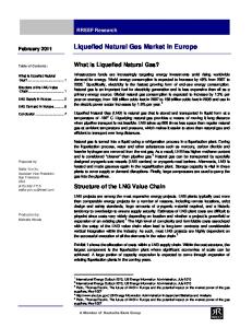
• Strong seasonal demand • Graphic for the US Market (2003)

Millions

Seasonal Demand Aspects 3.0 Residential

2.5

Commercial

Industrial

Electric Power

2.0 1.5 1.0 0.5

MMcf 0.0

Jan

Feb

Mar

Apr

May

Jun

Jul

Aug

Sep

Oct

Nov

Dec

Electric Power 382,443 334,698 361,243 352,164 394,021 435,598 630,270 683,513 468,510 408,817 348,129 335,810 Industrial

686,025 640,202 615,171 574,328 556,416 508,348 572,719 577,497 561,221 601,231 595,609 650,261

Commercial

522,463 487,178 390,806 263,067 181,047 137,575 132,219 130,824 136,613 181,260 259,504 394,103

Residential

945,744 884,233 674,581 414,062 247,501 157,262 126,386 115,784 128,579 231,574 413,718 738,775

Transportation and Distribution •

Pipelines in the US

•

Source: http://www.inogate.org/html/maps/mapsgas.htm

LNG degasification process in Qatargas Source: http://www.qatargas.com.qa/lng/lng-process.htm

LNG Storage Tank

LNG transportation and distribution

Security escort for LNG tanker

LNG Ship Unloading at Terminal

Picture source: http://www.ferc.gov/for-citizens/lng.asp

Industry Background • Deregulation results (US) – Price determination • In regulated market, the price of the gas was regulated by government. Gas was traded under long-term contracts. • In the deregulated market, the price of the gas is determined by market itself. • Spot market contracts are used to maintain flexibility to take advantage of market imbalance conditions caused by uncertain factors.

– More agents competing noncooperatively and independently • Gas sales, transportation and storage were unbundled from interstate natural gas pipelines by FERC Order 636 issued in April 1992, which also converted interstate gas pipelines to open access transporters.

– Roles played by policy makers • Policy makers focus on the competition control instead of price control.

Summary of Energy Modeling Forum (EMF23) and DOE Natural Gas/Fossil Fuel Meetings • Rising importance of LNG vs. pipelines – Increased demand (e.g., China) and increased importance of natural gas • Environmental reasons • Price reasons

• World Markets as opposed to previously just continental ones – When should Russia send gas east to S. Korea/Japan/N. America or west to Europe? – Trinidad gas to N. America or Europe (can decide “on the fly”)

• Importance of Russian influence – Constrained Russian exports, constrained Russian imports to EU (scenarios to run)

• Gas Cartel? – Russia, Qatar, Iran (scenarios to run)

• • • •

Strategic, Game Theory Models Vs. Cost-Minimization Ones Scenario Analysis vs. Stochastic Equilibrium Models Modeling investment decisions in the context of market equilibria Tracking individual supply projects and/or building up supply curves

Natural Gas in the Headlines of the New York Times Dec/Jan • Natural Gas and Geo-Politics-Russia – “Dispute Over Natural Gas Prices in Ukraine,” NYT 12/16/05 – “Putin Offers 3-Month Extension of Ukraine’s Gas Subsidy,” NYT 12/31/05 – “Russia Cuts Off Gas to Ukraine in Cost Dispute,” NYT 1/2/06 – “Russia Restores Most of Gas Cut to Ukraine Line,” NYT 1/3/06 – “A Dispute Underscoreds the New Power of Gas,” NYT 1/3/06 – “Russian and Ukraine Reach Compromise on Natural Gas,” NYT 1/5/06 – “Envoys Say Gas Crisis Hurt West’s Relations with Russia,” NYT 1/5/06 – “Ukraine Concedes it Took Gas From Pipeline but Says it Had the Contractual Right, “NYT 1/3/06 – “Gas Halt May Produce Big Ripples in European Policy,” NYT 1/3/06 – “Ex-Premier of Ukraine Attacks Gas-Price Deal,” NYT 1/7/06 – “Europe Comes to Terms with Need for Russian Gas,” NYT 1/8/06 – “Ukraine is Increasingly Dependent on Gas from Turkmenistan,” NYT 1/10/06 – “Gazprom Builds Wealth for Itself, but Anxiety for Others,” NYT 1/13/06”

Natural Gas in the Headlines of the New York Times Dec/Jan • Natural Gas and Geo-Politics-Georgia and Qatar – “Qatar Finds A Currency of Its Own,” NYT, 12/22/05 – “Explosions in Southern Russia Sever Gas Lines to Georgia,” NYT 1/23/06 – “Georgia Reopens Old Gas Line to East Post-Blast Storage,” NYT 1/24/06 – “Russia Gas Line Explosions Scare Europe,” NYT 1/26/06 – “Georgia, Short of Gas, Is Hit With a Blackout,” NYT 1/27/06

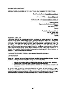
From “Russia Cuts Off Gas to Ukraine in Cost Dispute,” NYT 1/2/06

Min. gas price/1000 m3

Problems with Russia

Ukraine, $220

Orange Revolution, aspires to join NATO & EU

Moldova, $160

Russia supports separatists; aspires to join EU

Estonia, $120

NATO member; has border disputes with Russia

Latvia, $120

NATO member

Lithuania, $120

NATO member

Armenia, $110

None

Azerbaijan, $110

Is building rival oil and gas pipelines

Georgia, $110

Rose Revolution; Russia supports separatists

Belarus, $47

None

Natural Gas in the Headlines of the New York Times Dec/Jan • Other Natural Gas Issues – Natural Gas for Diesel Fuel: • “A New Old Way to Make Diesel”, NYT 1/18/06, Qatar

– Price Questions on Gas Rights: • “As Profits Soar, Companies Pay U.S. Less for Gas Rights Energy Giants Report Different Sales Prices to Investors and Federal Government,” NYT 1/23/06 • “Data Sought on Royalties Paid for Gas,” NYT 1/24/06

Gas Industry Modeling Activities N. America and European Union Models) • Operational models (e.g., storage, production) • Some large-scale equilibrium models

Deterministic Models

European Natural Gas Market

Deregulated North American Natural Gas Market

• GASTALE (Gas Market

• NGTDM (Natural Gas Transmission and Distribution Module) and OGSM (Oil and Gas Supply Module) in NEMS (National Energy Modeling System), 1990s

System for Trade Analysis in a Liberalising Europe), an oligopolistic model of production and trade, 2000s

• GSAM (Gas Systems Analysis Model), late 1990s

Stochastic Models

• A stochastic dynamic NashCournot model by Haurie et al., 1987 • A stochastic Stackelberg Cournot model by DeWolf and Smeers, 1997

Complementarity Modeling Methodology (Zhuang and Gabriel) • NCP/VI: Nonlinear Complementarity Problem/Variational Inequality Problem – Market equilibrium with certain players strategic (e.g., US: marketers, EU: producers)

• Stochastic NCP/VI • Stochastic programming is the framework for modeling optimization problems that involve uncertainty. – Recourse method used to formulate the stochasticity faced by each agent.

Market Composition • Market players – – – – – –

Producers Pipeline operators Storage operators Peak gas operators Marketers/shippers (only strategic players) Consumers • • • •

Residential Commercial Industrial Electric power

Market Network • Production regions – Producers

• Consumption regions – – – –

Storage operators Peak gas operators Marketers Consumers

• Pipeline arcs connecting production and consumption regions • Note: no intermediate regions modeled

Market Network Flows in season 1 Flows in seasons 2 & 3 Flows in season 3 Flows in seasons 1,2 & 3

P1

P2

CP1

CP2

MC1

RC1

RC2

PC1

RD1 CD1 ID1 ED1

RD2 CD2 ID2 ED2

C1

MC2

PC2 C2

Seasonality • Season 1 (low demand season) – April – October

• Season 2 (high demand season) – November, December, February, March

• Season 3 (peak demand season) – January

Recourse Method • Two-stage recourse program – First-stage: first-stage decision before the realization of the uncertainty – Random event occurs – Second-stage: recourse decision to compensate for any adverse effects that might have been experienced as a result of the firststage decision – Maximize/minimize the profit/cost of the first-stage decision plus the expected profit/cost of the recourse decision.

• Multistage recourse program – when the decision problem involves a sequence of decisions that react to outcomes that evolve over time

Scenario Tree of Demand Scenario

High

D 3,1 = 2

High D 2,1 = 2

High D

1,1

=2

0.4

Low D 2,1 = 1

0

s=0 t=0 y=0

D 1,1 = 1

High D

2,1

=2

2

8

9

Low D

3,1

=1

10

4

0.16

High

D 3,1 = 2

11

5

0.045

Low 3,1

12

=1

6

0.135

Low

D 3,1 =High 2

6

13 0.21

14 0.21

t=2 y=1 s=2

7

Low D 3,1 = 1

Long-term contract decision s=1

3

0.04

D

0.42

t=1 y=1

2

0.09

D 3,1 = 2

0.18

D 2,1 = 1

First-stage decisions (Long-Term Decisions)

=1

5

0.6

First-Stage:

D

4 0.2

Low

Low 3,1

High

1

1

0.11

3 0.2

7

t=3 y=1 s=3

Second-Stage: Recource Decisions (Spot Marketcontract Decisions) Spot market decisions

8

Model S-NGEM • Long-term contract decision: first-stage decision – Supply assurance – Firm service – Reservation charges

• Spot market contract decision: recourse decision – Flexibility to secure gas at lower price – Swing service and baseload service

Players • Consumers – Residential and commercial sectors • Represented by stochastic demand functions as part of the marketer’s problem • No long-term contract

– Industrial and electric power sectors • Predetermined demand • Mostly long-term contract demand

• Regulated Players – Pipeline Operator • Regulated by FERC • Maximize the expected congestion fees of the pipeline subject to the pipeline capacity

Players • Non-strategic players – Producers, storage operators and peak gas operators • Price-takers in their own market and in other markets • Aware of the uncertain demand implicitly via the marketclearing conditions • Maximize the expected profits subject to engineering restrictions, production capacity and material balance constraints.

Players • Strategic players – Marketers • Nash-Cournot players for the residential and commercial sectors • Price-takers in the production, storage, peak gas, and transportation markets. • The only players aware of consumers’ uncertain behaviors via the demand functions in their objective functions. • Maximize expected profits subject to gas volume balancing restrictions

Model Structure • Model S-NGEM – Optimization problems for all players except consumers • Maximize Expected profits • subject to Engineering and other constraints

– System Constraints • Market-clearing conditions for both the long-term and spot markets

• Model S-NGEM is an instance of a Mixed Nonlinear Complementarity Problem (MiCP). – Assumptions: • Convex, continuously differentiable cost functions • Concave revenue functions • Positive marginal costs in the positive orthant

Theoretical Results • A price relationship for the long-term and spot market contracts. – Take the producer as an example,

Conditions

Conclusions

(a)

≥

(b)

≤

(a) + (b)

=

– Similar relationship established for pipeline operators, peak gas operators and storage operators.

Sample Network • Example network: – Two production nodes • One producer at each production node

– Two consumption nodes, each consumption node has • • • •

One storage operator One peak gas operator Two marketers Four demand sectors

– Four pipelines connecting these four nodes

• Time horizon: One year with three seasons

C1

M1 M2

P1

C2

R1

R2

RD1 CD1 ID1 ED1

RD2 CD2 ID2 ED2

M3 M4

P2

Data Set • Deterministic Parameters – Capacities for all players – Cost functions for all players – Long-term demand for ID1, ID2, ED1 and ED2

• Stochastic Parameters – Spot market demand for ID1, ID2, ED1 and ED2 – Coefficients of the demand functions for RD1, RD2, CD1 and CD2 – Random demand at the two consumption nodes were assumed independent.

Computation • Linear complementarity problem (LCP) of 6,186 variables – 142 first-stage variables – 6,044 recourse variables

• GAMS/PATH as the solver • CPU time: from 5 to 20 seconds on a PC computer with a 2.26GHz Intel® Pentium®4 Processor and 1.0GB of memory

Case Studies • • • •

Base Case Case 1: low demand, low price scenario Case 2: high demand, high price scenario Case 3: perfect competition scenario

Expected Profits and Surplus

Wait-and-See Solution • WS: wait-and-see solution – Stochastic Program • WS = – where

is the solution to

– Stochastic Equilibrium Program • WSi =

for player i

– where is the solution to a Nash equilibrium problem which simultaneously maximizes all the players’ profits given other players’ decisions, that is, for each player i

Here-and-Now Solution • RP: here-and-now solution – Stochastic Program • RP = – whose solution is

– Stochastic Equilibrium Program • RPi =

for player i

– where is the solution to a stochastic Nash equilibrium problem which simultaneously maximizes all the players’ expected profits given other players’ decisions, that is, for each player i

EEV • EV: mean value ( ξ ) problem, whose solution is x(ξ ) • EEV: Expected result of using x(ξ ) – Stochastic Program • EEV = – where x(ξ ) is the solution to

– Stochastic Equilibrium Program • EEVi =

for player i

– where x(ξ ) is the solution to a Nash equilibrium problem which simultaneously maximizes all the players’ profits given other players’ decisions, that is, for each player i

Value of Stochastic Solution • Stochastic Program – RP: here-and-now solution • RP =

– Solve an expected value problem, EV= , whose solution is x(ξ ) – EEV: the expected result of using the EV solution x(ξ ) • EEV = – VSS: Value of Stochastic Solution • VSS = RP – EEV ≥ 0 • Measures the cost of using the expectation of the uncertainty thus ignoring the stochastic elements in the decision making process.

Value of Stochastic Solution • Stochastic Equilibrium Program – Define zi(x, ξ) as the profit or surplus function for player i, • x is the decision variable, • ξ is the random variable.

– Solve the stochastic equilibrium model, the solution is x* – RPi = for player i – Solve an expected value (EV) problem of above stochastic equilibrium problem, the solution is x(ξ ) – EEVi= for player i – VSSi = RPi – EEVi for each player i

EVPI and VSS • Stochastic Program – EEV ≤ RP ≤ WS – EVPI = WS – RP ≥ 0 • Measures the maximum amount a decision maker would pay in return of the complete information about the future.

– VSS = RP – EEV ≥ 0 • Measures the cost of using the expectation of the uncertainty thus ignoring the stochastic elements in the decision making process.

• Stochastic Equilibrium Program – For each player i • EVPIi = WSi – RPi • VSSi = RPi – EEVi

EVPI Player

Base Case

Case 1

Case 2

Case 3

Producer C1

-0.1

-0.4

-2.0

0.9

Producer C2

-0.5

-0.5

-4.3

-0.4

Storage Operator R1

0.4

0.1

4.1

1.2

Storage Operator R2

0.4

0.1

4.4

1.4

Peak Gas Operator P1

0.0

0.0

0.5

0.3

Peak Gas Operator P2

0.0

0.0

0.5

0.3

Marketer M1

0.1

0.2

-0.3

0.0

Marketer M2

0.1

0.2

-0.3

0.0

Marketer M3

0.1

0.3

-0.7

0.0

Marketer M4

0.1

0.3

-0.7

0.0

Producer Surplus

-0.3

0.3

1.2

3.7

Residential Surplus RD1

0.2

0.3

-0.4

-0.6

Residential Surplus RD2

0.1

0.4

-0.8

-0.9

Commercial Surplus CD1

0.2

0.2

-0.2

-0.3

Commercial Surplus CD2

0.1

0.3

-0.5

-0.5

Consumer Surplus

0.6

1.2

-1.9

-2.3

Numerical Values of VSS Player

Base Case

Case 1

Case 2

Case 3

Producer C1

-0.3

-0.5

27.6

-5.7

Producer C2

4.8

3.2

45.7

17.0

Storage Operator R1

0.0

0.3

5.9

2.0

Storage Operator R2

-0.4

0.0

4.4

-0.3

Peak Gas Operator P1

-0.1

-0.1

1.7

0.8

Peak Gas Operator P2

0.1

0.0

1.5

0.6

Marketer M1

4.4

3.5

2.7

0.0

Marketer M2

4.4

3.5

2.7

0.0

Marketer M3

3.6

2.6

3.3

0.0

Marketer M4

3.6

2.6

3.3

0.0

Producer Surplus

20.10

15.5

98.5

14.6

Residential Surplus RD1

5.7

4.5

4.7

2.9

Residential Surplus RD2

4.3

3.3

4.7

5.6

Commercial Surplus CD1

2.9

2.5

0.7

-0.1

Commercial Surplus CD2

2.8

2.0

1.8

3.2

Consumer Surplus

15.7

12.3

11.9

11.6

Value of Stochastic Solution • Observations – VSSi ≥ 0 does not hold for every player in the stochastic equilibrium program. – VSSi ≥ 0 holds for all marketers in all cases. – VSSi ≥ 0 holds for the producer and consumer surplus in all cases.

EVPI and VSS • Conclusions – The relationship EEVi ≤ RPi ≤ WSi does not hold for a stochastic equilibrium program.

Conclusions & Future Work • Summary of Work: – Stochastic NCP model of natural gas market developed – Theoretical results concerning relationship between long-term and expected spot market prices developed – Model run on several cases, initial exploration of VSS, verification of results on a small-scale duopoly

Conclusions & Future Work • Future Work: – To further explore the concept of the value of a stochastic solution (VSS) for a stochastic equilibrium program – Development of specialized algorithms to solve stochastic NCP equilibrium problem and testing on large-scale problems