N. Gregory Mankiw – Principles of Economics Chapter 6. SUPPLY, DEMAND, AND GOVERNMENT POLICIES Solutions to Problems and Applications 1.

If the price ceiling of $40 per ticket is below the equilibrium price, then quantity demanded exceeds quantity supplied, so there will be a shortage of tickets. The policy decreases the number of people who attend classical music concerts, since the quantity supplied is lower because of the lower price.

2.

a.

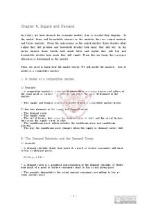
The imposition of a binding price floor in the cheese market is shown in Figure 3. In the absence of the price floor, the price would be P1 and the quantity would be Q1. With the floor set at Pf, which is greater than P1, the quantity demanded is Q2, while quantity supplied is Q3, so there is a surplus of cheese in the amount Q3 – Q2.

b.

The farmers’ complaint that their total revenue has declined is correct if demand is elastic. With elastic demand, the percentage decline in quantity would exceed the percentage rise in price, so total revenue would decline.

c.

If the government purchases all the surplus cheese at the price floor, producers benefit and taxpayers lose. Producers would produce quantity Q3 of cheese, and their total revenue would increase substantially. But consumers would buy only quantity Q2 of cheese, so they are in the same position as before. Taxpayers lose because they would be financing the purchase of the surplus cheese through higher taxes.

Figure 3 3.

a.

The equilibrium price of Frisbees is $8 and the equilibrium quantity is 6 million Frisbees.

1

Chapter 6

4.

b.

With a price floor of $10, the new market price is $10 since the price floor is binding. At that price, only 2 million Frisbees are sold, since that’s the quantity demanded.

c.

If there’s a price ceiling of $9, it has no effect, since the market equilibrium price is $8, below the ceiling. So the equilibrium price is $8 and the equilibrium quantity is 6 million Frisbees.

a.

Figure 4 shows the market for beer without the tax. The equilibrium price is P1 and the equilibrium quantity is Q1. The price paid by consumers is the same as the price received by producers.

Figure 4

Figure 5 b.

When the tax is imposed, it drives a wedge of $2 between supply and demand, as shown in Figure 5. The price paid by consumers is P2, while the price received by producers is P2 – $2. The quantity of beer sold declines to Q2.

Chapter 6

5.

Reducing the payroll tax paid by firms and using part of the extra revenue to reduce the payroll tax paid by workers would not make workers better off, because the division of the burden of a tax depends on the elasticity of supply and demand and not on who must pay the tax. Since the tax wedge would be larger, it is likely that both firms and workers, who share the burden of any tax, would be worse off.

6.

If the government imposes a $500 tax on luxury cars, the price paid by consumers will rise less than $500, in general. The burden of any tax is shared by both producers and consumers⎯the price paid by consumers rises and the price received by producers falls, with the difference between the two equal to the amount of the tax. The only exceptions would be if the supply curve were perfectly elastic or the demand curve were perfectly inelastic, in which case consumers would bear the full burden of the tax and the price paid by consumers would rise by exactly $500.

7.

a.

b.

It doesn’t matter whether the tax is imposed on producers or consumers⎯the effect will be the same. With no tax, as shown in Figure 6, the demand curve is D1 and the supply curve is S1. If the tax is imposed on producers, the supply curve shifts up by the amount of the tax (50 cents) to S2. Then the equilibrium quantity is Q2, the price paid by consumers is P2, and the price received (after taxes are paid) by producers is P2 – 50 cents. If the tax is instead imposed on consumers, the demand curve shifts down by the amount of the tax (50 cents) to D2. The downward shift in the demand curve (when the tax is imposed on consumers) is exactly the same magnitude as the upward shift in the supply curve when the tax is imposed on producers. So again, the equilibrium quantity is Q2, the price paid by consumers is P2 (including the tax paid to the government), and the price received by producers is P2 – 50 cents.

Figure 6 The more elastic is the demand curve, the more effective this tax will be in reducing the quantity of gasoline consumed. Greater elasticity of demand means that quantity falls more in response to the rise in the price of gasoline. Figure 7 illustrates this result. Demand curve D1 represents an elastic demand curve, while demand curve D2 is more inelastic. To get the same tax wedge between demand and supply requires a greater reduction in quantity with demand curve D1 than for demand curve D2.

Chapter 6

Figure 7

8.

c.

The consumers of gasoline are hurt by the tax because they get less gasoline at a higher price.

d.

Workers in the oil industry are hurt by the tax as well. With a lower quantity of gasoline being produced, some workers may lose their jobs. With a lower price received by producers, wages of workers might decline.

a.

Figure 8 shows the effects of the minimum wage. In the absence of the minimum wage, the market wage would be w1 and Q1 workers would be employed. With the minimum wage (wm) imposed above w1, the market wage is wm, the number of employed workers is Q2, and the number of workers who are unemployed is Q3 - Q2. Total wage payments to workers are shown as the area of rectangle ABCD, which equals wm times Q2.

Chapter 6

Figure 8 b.

An increase in the minimum wage would decrease employment. The size of the effect on employment depends only on the elasticity of demand. The elasticity of supply doesn’t matter, because there’s a surplus of labor.

c.

The increase in the minimum wage would increase unemployment. The size of the rise in unemployment depends on both the elasticities of supply and demand. The elasticity of demand determines the quantity of labor demanded, the elasticity of supply determines the quantity of labor supplied, and the difference between the quantity supplied and demanded of labor is the amount of unemployment.

d.

If the demand for unskilled labor were inelastic, the rise in the minimum wage would increase total wage payments to unskilled labor. With inelastic demand, the percentage decline in employment would be less than the percentage increase in the wage, so total wage payments increase. However, if the demand for unskilled labor were elastic, total wage payments would decline, since then the percentage decline in employment would exceed the percentage increase in the wage.

Chapter 6 9.

a.

Figure 9 shows the effect of a tax on gun buyers. The tax reduces the demand for guns from D1 to D2. The result is a rise in the price buyers pay for guns from P1 to P2, and a decline in the quantity of guns from Q1 to Q2.

Figure 9 b.

Figure 10 shows the effect of a tax on gun sellers. The tax reduces the supply of guns from S1 to S2. The result is a rise in the price buyers pay for guns from P1 to P2, and a decline in the quantity of guns from Q1 to Q2.

Figure 10

Chapter 6 c.

Figure 11 shows the effect of a binding price floor on guns. The increase in price from P1 to Pf leads to a decline in the quantity of guns from Q1 to Q2. There is excess supply in the market for guns, since the quantity supplied (Q3) exceeds the quantity demanded (Q2) at the price Pf.

Figure 11 d.

10.

a.

Figure 12 shows the effect of a tax on ammunition. The tax on ammunition reduces the demand for guns from D1 to D2, because ammunition and guns are complements. The result is a decline in the price of guns from P1 to P2, and a decline in the quantity of guns from Q1 to Q2.

Figure 12 Programs aimed at making the public aware of the dangers of smoking reduce the demand for cigarettes, shown in Figure 13 as a shift from demand curve D1 to D2. The

Chapter 6 price support program increases the price of tobacco, which is the main ingredient in cigarettes. As a result, the supply of cigarettes shifts to the left, from S1 to S2. The effect of both programs is to reduce the quantity of cigarette consumption from Q1 to Q2.

Figure 13

11.

b.

The combined effect of the two programs on the price of cigarettes is ambiguous. The education campaign reduces demand for cigarettes, which tends to reduce the price. The tobacco price supports raise the cost of production of cigarettes, which tends to increase the price.

c.

The taxation of cigarettes further reduces cigarette consumption, since it increases the price to consumers. As shown in the figure, the quantity falls to Q3.

a.

The effect of a $0.50 per cone subsidy is to shift the demand curve up by $0.50 at each quantity, since at each quantity a consumer's willingness to pay is $0.50 higher. The effects of such a subsidy are shown in Figure 14. Before the subsidy, the price is P1. After the subsidy, the price received by sellers is PS and the effective price paid by consumers is PD, which equals PS minus 50 cents. Before the subsidy, the quantity of cones sold is Q1; after the subsidy the quantity increases to Q2.

Figure 14

Chapter 6

b.

Because of the subsidy, consumers are better off, since they consume more at a lower price. Producers are also better off, since they sell more at a higher price. The government loses, since it has to pay for the subsidy.