Remote Sensing: Advanced Topics
Hyperspectral remote sensing
MODULE – 9 LECTURE NOTES – 4 HYPERSPECTRAL REMOTE SENSING
1. Introduction Hyperspectral remote sensing, also known as imaging spectroscopy is a relatively new technique used by researchers and scientists to detect terrestrial vegetation, minerals and land use/land cover mapping. Though this data has been available since 1983 onwards, their widespread use is initiated primarily due to a number of complicated factors serving applications in various fields of engineering and science. Spectroscopy has been used by scientists, especially physicists for many years for identifying material composition. Many techniques employed for analyzing reflectance spectra have been developed in the field of analytical chemistry. It detects individual absorption features based on the chemical bonds in solids/liquids/gases. Technological advancements have enabled imaging spectroscopy to be extended beyond laboratory settings to satellites so that its applications can be focused over a global extent. In some books, hyperspectral has been used synonymously with the work imaging spectrometer. Within the electromagnetic spectrum, it is well known that not all spectral bands are available for remote sensing purposes. Atmospheric windows or regions in which remote sensing is possible tend to separate the absorption bands. Hyperspectral images are measurements acquired within these atmospheric windows. The technique of hyperspectral remote sensing combines imaging and spectroscopy within a single system thereby resulting in large data sets that require sophisticated processing methods. Generally, hyperspectral data sets will be composed of about 100 to 200 spectral bands possessing relatively narrow bandwidths unlike the multispectral data sets which possess just 5-10 bands of relatively larger bandwidths. Some examples of hyperspectral sensors are Hymap or Hyperspectral Mapper used for airborne imaging and Airborne Visible/ Infrared Imaging Spectrometer (AVIRIS) first deployed by NASA in early 1980s.
D Nagesh Kumar, IISc, Bangalore
1
M9L4
Remote Sensing: Advanced Topics
Hyperspectral remote sensing
Figure 1: Multispectral Vs Hyperspectral Remote Sensing
Hyperspectral imagery can be visualized in 3D space as a data cube of spatial information collected in the X, Y plane wherein spectral information captured in various bands are represented in the Z direction. This allows us to look at hyperspectral images in two ways; one focusing on the spatial patterns in x-y plane and second is to analyse the properties of a specific location/pixel point along the Z direction.
Figure 2: Visualization of a hyperspectral data cube D Nagesh Kumar, IISc, Bangalore
2
M9L4
Remote Sensing: Advanced Topics
Hyperspectral remote sensing
Figure 3: Concept of an Imaging Spectrometer
2. Hyperspectral sensor systems One of the major issues with hyperspectral analysis is the lack of high quality data sets for most areas of interest. This situation is changing rapidly with the availability of hyperspectral aircraft sensors flown for both government and commercial purposes. Some of the initial studies involving hyperspectral sensing was conducted with data acquired using the Airborne Imaging Spectrometer (AIS) which collected data using 128 bands which were approximately 9.3 nm wide. The system which operated from an altitude of 4200 m above terrain resulted in a total of 32 narrow swath pixels with a resolution of approximately 8 x 8 m. Color composites can be generated using hyperspectral images by displaying three bands at a time, with one band displayed as blue, one as green and one as red. Commonly, the images of all bands will be displayed in isometric view wherein data is thought of as a cube. The top and side of the cube will represent color coded reflectance values corresponding to the 224 spectral bands. The very first commercially made available hyperspectral scanner was the Compact Airborne Spectrographic Imager (CASI) which collected data using 288 bands between 0.4 and 0.9 D Nagesh Kumar, IISc, Bangalore
3
M9L4
Remote Sensing: Advanced Topics
Hyperspectral remote sensing
m with an instantaneous field of view of 1.2 mrad. This system was used in combination with global positioning system GPS) so as to correct for aircraft altitude variations. The Advance Airborne Hyperspectral Imaging Spectrometer (AAHIS) is another commercially produced hyperspectral scanner which captures information in around 288 channels within 0.40 to 0.90 m ranges. Another such instrument is the Airborne Visible-Infrared Imaging Spectrometer (AVIRIS) that collects data using 224 bands which are approximately 9.6 nm wide between bands 0.40 and 2.45 m . This resulted in a ground pixel resolution of approximately 20 m. As a follow up of AVIRIS, the Hyperspectral Digital Image Collection Experiment (HYDICE) was developed with the sole intention to advance hyperspectral scanner system with a higher spatial resolution. The TRW Imaging Spectrometer was developed for use in both aircraft and spacecraft which uses around 384 channels operating in the wavelength range between 0.40 to 0.25 m range. The HyMap (Hyperspectral Mapping) system, the first commercially available sensor to provide high spatial and spectral resolution data is built by Integrated Spectronics and is capable of sensing upto 200 bands. Its availability has tapped the potential of commercial use of airborne imaging spectrometry. It is possible for the airborne hyperspectral data to generate spectral reflectance curves for minerals that are similar to those generated within laboratory settings. With the successful use of hyperspectral imagery from AVIRIS and HyMap, global availability of high quality hyperspectral data has been given priority to cater to the needs of various applications in engineering and sciences division. As a direct consequence, several satellite systems are under development like Orbview-4, AIRES-1 etc. Orbview-4 is capable of imaging earth at a spatial resolution of one meter panchromatic and four meter multispectral which includes an imaging instrument comprising of 280 channels. ARIES-1 is an Australian Resource Information and Environment Satellite, flying in low earth orbit and carrying a hyperspectral sensor using reflected visible and infrared light. It has 32 contiguous bands providing commercial use to the international remote sensing market place.
3. Hyperspectral Image Analysis Even though hyperspectral sensors enable to identify and discriminated between different earth surface features, these suffer from disadvantages. Some of these are an increased volume of data to be processed, poor signal to noise ratios and atmospheric interference. Hence, analysis of hyperspectral images relies on physical and biophysical models than on
D Nagesh Kumar, IISc, Bangalore
4
M9L4
Remote Sensing: Advanced Topics
Hyperspectral remote sensing
other statistical techniques. Atmospheric gases and aerosols tend to absorb light at particular wavelengths. Atmospheric attenuation exists in the form of scattering (addition of extraneous source of radiance into the sensor’s field of view) and absorption (negation of radiance). As a consequence, the radiance registered by a hyperspectral sensor cannot be compared to imagery procured at other times/locations. Hyperspectral image analysis techniques are derived using the field of spectroscopy which relates the molecular composition of a particular material with respect to the corresponding absorption and reflection pattern of light at individual wavelengths. These images need to be subjected to suitable atmospheric correction techniques so that the reflectance signature of each pixel is compared with the spectra of known materials. The spectral information of known materials like minerals, soils, vegetation types etc will usually be collected in laboratory settings and stored as “libraries”. Different means are employed to compare the reference spectra with the obtained spectral reflectance. Previously, individual absorption features were identified in the image by selecting one spectral band occurring in the low point and two bands located on either side of the absorption feature. This method will be subjected to noise in the image data. Also, it will be difficult to deal with overlapping absorption features. With an increase in the computational facilities, this approach has advanced to comparison of entire spectral signatures rather than individual absorption features within a signature. Another method is spectrum ratioing which is, dividing every reflectance value in the reference spectrum by the respective value of the image spectrum. The disadvantage of this method is that it fails when the average brightness of the image spectrum is higher/lower than the average brightness of the reference spectrum as is observed over a topographically shaded slope. Another technique commonly adopted is the spectral angle mapping (SAM). This method considers an observed reflectance spectrum as a vector within a multidimensional space. It allows the number of dimensions to be equal to the number of spectral bands. The advantage of this method is that even with an increase/decrease in the overall illumination, the vector length will increase/decrease but its angular orientation will remain constant. In order to compare two spectra, it is required that the multidimensional vectors are defined for each spectrum and the angle between the two vectors be calculated. An angle value smaller than the given tolerance level will result in a match (between the library reference spectrum and the image pixel spectrum) even if one spectrum is brighter than the other. For a hyperspectral sensor with 300 or more bands, it becomes difficult for humans to visualize the dimensionality of space wherein vectors are located. Different
D Nagesh Kumar, IISc, Bangalore
5
M9L4
Remote Sensing: Advanced Topics
Hyperspectral remote sensing
methods exist to process hyperspectral imagery. Though it is not possible to cover the entire topic in this module, one such method is discussed below. 3.1 Derivative Analysis A digital image can be represented in terms of a 2 dimensional function that has a pixel value (DN number) associated with each row (r) and column (c) so that pixel value=f(r,c) . But this function is not continuous for every possible values of r and c and hence is non differentiable in nature. Hence, to estimate the rate of change at a particular point, the method of differences is adopted. Assume that the spectral reflectance curve of a target is collected by a hyperspectral sensor. Let yi and yj denote the adjacent, discrete reflectance values on this curve at wavelengths xi and xj such that the first difference value can be given by the expression y yi yj x xi xj
The first difference essentially gives the rate of change of function y with respect to its distance along the x axis. Similarly, we can also obtain the second difference which gives the rate of change of slope with distance along the x axis. This shows how rapidly the slope is changing. The first and second differences calculated for one dimensional spectra or 2 dimensional images provide means to approximate the derivatives of a discrete function which cannot be calculated. The analysis of position and magnitude of absorption bands in the pixel spectrum can be estimated using the derivative analysis. The derivative methods tend to amplify any noise if present in the data. Hence, various methods of noise removal are applied to hyperspectral data ranging from simple filtering approaches to more complex wavelet based methods.
3.2 Atmospheric Correction As mentioned earlier, atmosphere influences remote sensing measurements by the two major phenomenons of scattering and absorption. The effects of absorption are more pronounced due to water vapor with smaller contributions from ozone, carbon dioxide etc, The main step to analyse hyperspectral imagery is to convert the data into reflectance values such that the individual spectra can be compared with either laboratory libraries or field data. The laboratory setting enables provision to calibrate the initial wavelengths. For example, in the visible and near infrared regions of the electromagnetic spectrum, the narrow atmospheric
D Nagesh Kumar, IISc, Bangalore
6
M9L4
Remote Sensing: Advanced Topics
Hyperspectral remote sensing
bands at 0.69, 0.72 and 0.76 m can be utilized to calibrate wavelengths. Several methods exist to empirically correct the atmospheric effects. Some techniques involve subtraction of average normalized radiance value of each channel from each normalized spectrum resulting in a residual image. Another method dealing with calculating the internal average relative reflectance involves estimating an average spectrum for an entire imaging spectrometer dataset. This can then be used for dividing each spectrum in the data set by the average spectrum. The point to be noted is that all of these methods tend to eventually produce images and spectra that have characteristics similar to reflectance. Hence, they result in relative reflectance i.e., reflectance relative to a reference spectrum and not absolute reflectance. The disadvantage associated with such practices is the presence of artifacts that gets incorporated as the reference spectrum themselves might possess spectral characteristics related to specific absorption features. On the positive note, conversion to an apparent reflectance doesn’t require a priori knowledge regarding the site. To circumvent these issues, a standard area on the ground can be used to correct the data to reflectance wherein two or more ground locations can be chosen with albedos which span a wider range. Then, multiple pixels can be selected within the data set associated with each ground target which can be incorporated within a linear regression setting to estimate the gain and offsets required to convert the digital number to reflectance values. Solution of this equation will provide estimates of the standard error for each parameter at each wavelength. The final step in reflectance correction is to multiply the instrument digital number values with the gain factor and to add the corresponding offset values. This will essentially remove atmospheric effects of scattering and absorption, geometry effects and other instrument related artifacts. Model based atmospheric correction techniques are also being developed like the Atmospheric Removal Program (ATREM). Here, a three channel ratioing approach is undertaken to estimate the water vapor on a pixel by pixel basis using the AVIRIS data. For different water vapor amounts, a number of theoretical water vapor transmittance spectra can be calculated using radiative transfer modeling. Such a modeled spectra can be run through the three channel ratioing method and used to generate look up tables of water vapor concentrations. These values can be used to convert the AVIRIS apparent reflectance measurements to total column water vapor. As a result, we obtain the spatial distribution of various water vapor concentrations for each pixel of AVIRIS data. This image can then be used along with transmittance spectra derived for each of the atmospheric gases to produce a scaled surface reflectance. The currently available models to correct atmospheric effects
D Nagesh Kumar, IISc, Bangalore
7
M9L4
Remote Sensing: Advanced Topics
Hyperspectral remote sensing
enable to quantitatively derive the physical parameters and analyze data without a priori knowledge.
4. Applications
a) Land use applications: Generally, remotely sensed images will be processed using digital image processing methods like supervised and unsupervised classification.
With the
availability of hyperspectral data of increased spatial and spectral resolution, the potential for land use classification has increased manifold. This imagery acquired in various spectral bands complement the existing information from traditional remotely sensed images. A special mention is to be made about vegetation mapping as it has unique spectral signatures during various stages of its growth that varies with species type. Improved classification is ensured using the hyperspectral imagery owing to the improved quality in the reference spectra.
b) Ecological Applications: Vegetation indices derived using hyperspectral sensors conclude better and more sensitive than those derived using optical images. Knowledge regarding the reflectance spectrum of vegetation is crucial for many applications. The biophysical factors which affect the spectrum of active vegetation are the leaf chemistry which is responsible for the absorption characteristics of leaf spectrum in the visible wavebands. Different vegetation has different spectral reflectance curves which can be characterized using vegetation indices. These indices are essentially ratios that measure the steepness of the red-infrared region of the spectral reflectance curve but not its position within the spectrum. Using data from hyperspectral sensor, it is possible to characterize this steep rise in the reflectance curve in terms of a single wavelength.
c) Water Quality Hyperspectral images have been used to assess the water quality in many open water aquatic ecosystems indirectly by classifying trophic status of lakes, characterizing algal blooms, predicting total ammonia concentrations to monitor wetland water quality changes. Using remotely sensing images, the chlorophyll content is usually estimated which in turn can be used for monitoring algal content and therefore water quality. Due to the narrow contiguous bands, hyperspectral images allow for a better detection of chlorophyll and algae.
D Nagesh Kumar, IISc, Bangalore
8
M9L4
Remote Sensing: Advanced Topics
Hyperspectral remote sensing
d) Flood Detection Previously, though satellite remote sensing enabled monitoring of inundated areas during floods or any other natural calamity, near real time flood detection was not possible. To provide real time information about natural disasters like floods, timely information of water conditions is required at sufficient spatial and temporal resolutions. Using sensors such as Hyperion on board the EO-1 satellite, this is made possible. Many studies of USGS and NASA utilize satellite based observations of precipitation, topography, soil moisture, evapotranspiration etc into early warning systems. The hydraulic information obtained using remotely sensed images can be applied in flood routing studies to generate flood wave in a synthetic river channel. Research is also underway to estimate river discharge using satellite microwave sensors with an aim to improve warning systems.
e) Evapotranspiration (ET): Information regarding evapotranspiration is crucial for various applications involving irrigation, reservoir loss study, runoff prediction, climatology etc to name a few. Even though it cannot be measured by direct means, hyperspectral sensors offer means to estimate components of energy balance algorithms for spatially mapping ET values. Typically AVHRR and MODIS data are used to estimate evaporative fraction which is a ratio of ET and available radiant energy. More information can be obtained in Batra et al (2006), Eichinger et al 2006 etc. Analysis of hyperspectral images possesses great potential to advance the quality of spectral data obtained by sensing earth surface features. Research is currently underway to optimize the analysis of large volumes of hyperspectral imagery. As mentioned earlier, this is crucial for various applications such as identification of aerosols, gas plumes etc.
f) Geological Applications Hyperspectral remote sensing has great potential not only to identify but also to map specific chemical and geometric patterns of land which can be relied to identify areas with economically valuable deposits of minerals/oils.
D Nagesh Kumar, IISc, Bangalore
9
M9L4
Remote Sensing: Advanced Topics
Hyperspectral remote sensing
Figure 4: Applications of hyperspectral remote sensing
D Nagesh Kumar, IISc, Bangalore
10
M9L4
Remote Sensing: Advanced Topics
Hyperspectral remote sensing
Bibliography
1.
Chandrasekhar, S (1950), Radiative Transfer. Oxford University Press, Oxford, 393 pp.
2.
John R. Jensen, 1996, Introductory Digital Image Processing, Prentice Hall
3.
Lillesand T. M. & Kiefer R. W., 2000. Remote Sensing and Image Interpretation, 4th ed. Wiley & Sons.
4.
Paul. MK. Mather, 2004, Computer Processing of Remotely- Sensed Images, Wiley & Sons.
5.
Volchok, B. A. and M. M. Chernyak (1969), Transfer of microwave radiation in clouds and precipitation. Transfer of Microwave Radiation in the Atmosphere, NASA TT F-590, 90-97.
6.
Wilheit, T. T., Chang, A. T. C., Rao, M. S. V., Rodgers, E. B. and Theon, J. S (1977), A satellite technique for quantitatively mapping rainfall rates over the oceans., J. Appl. Meteorol., 16, 551-560.
D Nagesh Kumar, IISc, Bangalore
11
M9L4