Modeling the North American Market for Natural Gas Liquids by Robert E Brooks, Founder & President RBAC, Inc. 14930 Ventura Blvd, Suite 210, Sherman Oaks CA 91403 Tel: 818-501-7300, Fax: 818-501-7304, [email protected] Abstract This paper concerns NGL-NA™, a new model designed to analyze and forecast market fundamentals in the North America natural gas liquids (NGL) market. A principal impetus for this model is the expanding production of natural gas and natural gas liquids due to the “shale gas revolution”. This phenomenon has stressed existing NGL infrastructure and caused unanticipated declines in NGL prices. The industry requires a realistic scenario analysis tool to help it identify and evaluate investment opportunities in this fast growing but risky market. This is a model of a complex multi-commodity market. Upon production, raw natural gas is treated to remove contaminants such as carbon dioxide, hydrogen sulfide, and nitrogen, resulting in “wet” natural gas. This is processed to separate “dry” natural gas, mostly methane, from natural gas liquids. The dry gas is moved by pipeline to residential, commercial, industrial, and power plant customers downstream. The remaining liquid is called NGL Mix or Y-Grade NGL. It consists primarily of ethane, propane, iso-butane, normal-butane, and “natural gasoline” (pentanes, hexanes, etc.) Y-Grade is moved primarily by pipeline, but in some cases by rail or truck, to “fractionation” plants where it is separated into its various “purity products”. Each of these has its own markets. One of the most important of these is “petchem” plants, also known as olefin plants or “steam crackers”. These plants convert NGL’s into ethylene, propylene, butadiene, and other chemicals which are important precursor products to the plastics and synthetic rubber industries. The paper describes the design of a multi-period, market-clearing model, solved as a piecewise linear program, using AMPL for model design and Gurobi for efficient solution. Though this specific implementation of the model covers North America, the NGL market, and the market for olefins made from NGLs, is global. Principles used in the development of this model can also be used in an extension to the global market.

Description of Market The NGL market originates with production of crude oil, condensate, and natural gas. This is a somewhat crude classification into three categories of a whole spectrum of hydrocarbons produced by the industry, from the heaviest and most complex (crude oil) to the lightest and simplest (natural gas). Condensate resides in the middle zone, consisting of those lighter hydrocarbons that are yet liquid at temperatures and pressures found on the ground above the formations from which they are produced. Any given well could produce one or more of these products which are then generally separated on the leasehold for transport to different markets. A well is usually classified by which of these three is its most predominant product. Crude oil produced in the US or imported from other countries is shipped to refineries via pipeline or rail car. Heavy crude such as that produced in the oil sands of Alberta requires NGL-NA is a trademark owned by RT7K, LLC, and is used with its permission.

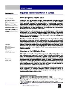
blending with lighter hydrocarbons to enable or improve transportability. The blending material is called diluent. This material may consist of condensate produced in the same or other fields or may be natural gas liquids produced by natural gas processing plants or even liquefied refinery gases produced by refineries. Condensate is shipped by pipe, rail, or possibly truck to refineries or to heavy oil fields or to “splitters” which separate the lighter natural gas liquids from the heavier hydrocarbons such as naphtha. From the splitters, the NGLs are then sent to fractionators and the naphtha to refineries. Condensate is sometimes sold as diluent. Natural gas is mostly methane but also contains ethane, propane, isobutane, normal butane, and “natural gasoline” (pentane, hexane, etc.) These are termed “natural gas liquids” even though all but natural gasoline are gaseous at room temperature and pressure. If the gas is very “dry”, it can be inserted directly into natural gas pipelines for transport to market. If it is “wet”, it is usually sent to natural gas processing plants where the liquids are separated from the dry gas. The exceptions occur when there is insufficient gas processing capacity or when NGL prices are too low to justify extraction. In these cases, producers sell the wet gas at dry gas prices, or extract only the heavier NGLs, and deliver the resulting gas to pipelines. Pipelines, however, limit the wetness of the gas so it will not adversely affect their operations. From the processing plant, dry gas is delivered to a gas pipeline and liquids can be loaded into mixed NGL (Y-Grade) pipelines or rail cars or trucks. Wetness of gas is measured in gallons of mixed NGLs per thousand cubic feet of wet gas (“GPM”). The following figure shows substantial regional variation in wetness of gas.

Figure 1: Natural Gas Liquids Content by Basin (National Petroleum Council, 2011)

2

Mixed NGLs are generally delivered to fractionation plants where the Y-Grade is separated into the individual “purity” products often labelled as C2, C3, N-C4, I-C4, and C5+. Both NGL Mix input and purity product output is stored in separate caverns in underground salt dome storage fields (or above ground tanks when volumes are small enough). Injection and withdrawal from these fields is accomplished using immiscible brine which is stored in above ground ponds when not injected underground. The amount of usable storage is limited by both the underground capacity and the above ground brine pond capacity. Each of these products has its own set of markets. Ethane is almost exclusively used in the manufacture of ethylene. Propane can be used for cooking and heating in areas where natural gas (methane) distribution is not available, in transportation, in agriculture and in ethylene production. Normal butane is used by oil refineries as blending material for gasoline and for making isobutane which is also a blending component. The demand for isobutane and normal butane in gasoline blending is quite seasonal. This is due to EPA regulations that impose RVP (Reid Vapor Pressure) restrictions during the summer months (typically Jun-Sep) in order to reduce transportation related air emissions. These summer restrictions increase the demand for iso-butane and correspondingly reduce the normal-butane demand for motor gasoline blending purposes. As ambient temperature changes occur during the fall and winter months, these restrictions are eased which allows for greater normal-butane blending (i.e. increasing normal-butane demand) into the motor gasoline pool and thereby reduces the demand for isobutane. Note that specialized “isomerization” units are also employed to convert normal butane to iso-butane to help satisfy this seasonal demand. Butane is also used to create butadiene, a chemical used in production of synthetic rubber. “Pentane +” or “natural gasoline” is typically used in gasoline blending but can also be used as diluent for heavy oil transportation. The market for diluent is growing due to higher bitumen production in the oil sands region of Alberta. Production of ethylene, propylene, butadiene, and other chemicals is accomplished in petrochemical plants known as “steam crackers”. More ethylene is produced worldwide than any other organic chemical. The composition of the inputs is controlled to yield the desired outputs. The table below (borrowed from a Wachovia Bank primer on NGLs) shows a representative example of the outputs associated with each unit of purity product NGLs from fractionators and naphtha and gasoil from refineries. Typical Steam Cracker Yields Based On Various Feedstocks Light Feeds Heavy Feeds (Yield by weight) Ethane Propane Butane Naphtha Gasoil Hydrogen & methane 13% 28% 24% 26% 18% Ethylene 80% 45% 37% 30% 25% Propylene 2% 15% 18% 13% 14% Butadiene 1% 2% 2% 5% 5% Mixed butenes 2% 1% 6% 8% 6% C5+ 2% 9% 13% 8% 7% Benzene 0% 0% 0% 5% 5% Toluene 0% 0% 0% 4% 3% Fuel oil 0% 0% 0% 2% 18% Feedstock Source: Chemistry of Petrochemical Processes. Sami Matar, Lewis Frederic Hatch Table 1: Typical Steam Cracker Yields by Feedstock

3

The principal product for all of these inputs is ethylene, with smaller amounts of propylene, and other by-products. Generally the hydrogen and methane gases produced are used to boil water to make the steam used in the cracking process. Demand for ethylene is the primary driver for the petchem industry as it is the principal ingredient for polyethylene, the most important starting product for production of plastics. About two-thirds of all propylene is used to make polypropylene, the second most important starting product in plastics. Though propylene is typically a by-product of ethylene production, propane dehydration plants (PDH) exist to produce “on-purpose” propylene. Similar BDH (butane dehydration) plants are used to make “on-purpose” butadiene.

NGL-NA Product Flow Model Figure 2 below shows the product flow model for NGL-NA. Nodes (circles) represent operations and arcs (directed arrows) represent product flow. The basic operations considered are Production (including separation and conditioning), Condensate Splitting, Crude Oil Refining, NGL Fractionation, and NGL Steam Cracking. Subsequent to any operation, the resulting product can be stored or moved to one or more of the other operations by pipeline, rail, truck, or barge. Implicit in the diagram below is that storage of both inputs and outputs can occur wherever some type of conversion operation occurs. Potential bottlenecks in the system are production and storage capacity in each operation in the supply chain as well as transportation between operations.

Figure 2: NGL-NA Product Flow Model Product can enter the system as imports or leave as exports using tankers. Imports and exports among the US, Canada, and Mexico are considered to be endogenous to the system 4

whereas those from or to other countries are computed as excess demand or supply in various regions. Import and export prices are exogenously set by the user as scenario assumptions.

Modeling Considerations Oil and Gas Production Levels of oil, gas, and condensate production are user inputs. These can be outputs from a natural gas market model scenario or any other source. North American oil production is an important input, because the changing quality of oil is already making a difference in terms of refinery outputs, including that of LPG (liquefied petroleum gas), a mixture of ethane, propane, and butane. Wet gas in each producing region is characterized by its chemical composition. This can be modeled as composition by weight or by wetness content (GPM, or gallons of liquids per thousand cubic feet of gas) and per cent composition of the liquids by weight. Assumptions about composition may change over time to reflect a trend toward greater dryness or wetness of the gas as the play is developed. However, model size grows proportionally with number of distinct compositions. Note: composition data is not generally available from public or industry sources. However, it can be inferred from data on natural gas and liquids production. Crude Oil Refining Crude oil comes in many different compositions. For the purposes of NGL-NA, we need to be able to characterize a variety of crudes produced and imported into North American refineries by their yields. The model must then be able to compute how much LPG is produced per barrel of each type of crude produced or imported and how much NGL purity product is needed for gasoline blending. This is clearly a very complex operation and is unique to each plant and crude used by each plant. The challenge for NGL-NA is generalizing this operation using a small number of parameters to adequately represent the process of converting a barrel of crude into those refined products which affect the NGL market, namely LPG and gasoline, as well as the required volume of butane and “natural gasoline” required for gasoline blending. Condensate Splitting Condensate can be utilized as is or can be “split” into light and heavy streams. The light steam is an NGL Mix and the heavy stream is composed of naphtha and other compounds. Each condensate is unique. In NGL-NA, each must be characterized in a reasonable way. This means the model will need parameters representing the split between light and heavy and some idea of the composition of the NGL mix. Gas Plant Processing The figure below gives a very good generalized picture of “gas processing”. It includes the separation operation discussed earlier under Oil and Gas Production, elimination of nonhydrocarbon compounds and elements such as water, CO2, sulfur, helium, and nitrogen (conditioning), removing methane from the resulting hydrocarbon stream and then “fractionating” the resulting mix into the five component NGL purity products. For the purpose of the NGL-NA model, the primary function of gas plant processing is separating wet gas into the dry gas (mostly methane) and mixed NGLs. That is, for our purposes, natural gas plant processing assumes non-hydrocarbon compounds have already been netted out of the initial 5

specification of “wet gas” production volume. And we assume that separation of the mixed NGLs occurs in a later process called “fractionation”.

Figure 3: Generalized Natural Gas Processing Schematic (EIA) There are several different types of gas processing plants, but their processes are usually categorized as absorption, refrigeration, or cryogenic expansion. Whereas absorption methods are excellent for extracting butanes, pentanes, and heavier products, they are less effective for the lighter products such as propane and ethane. Maximum ethane recovery is about 40%. Refrigeration plants are less efficient still, recovering most of the butane and natural gasoline but only about 30-50% of propane and none of the ethane. Cryogenic expansion is much more efficient at extracting propane and ethane. Cryogenic processes are able to improve extraction efficiency for ethane into the 90-95% range. Combining the composition of the gas delivered by gathering systems to the gas processing plants with the known recovery factors of each type of plant, one can compute the composition of the mixed NGLs resulting from processing. There is, however, one wrinkle in this calculation: ethane rejection. If the price of ethane is too low because it is in excess supply, then some processing plants can be operated so that some or most of the ethane is delivered to pipelines with the dry gas, rather than the NGL mix. For example, a cryogenic plant built by Thomas Russell Company has two modes of operation: ethane recovery mode removes 90-95% of the ethane whereas ethane rejection mode removes only about 11%. NGL-NA includes both options. It computes how much of each plant’s capacity is used in recovery mode and how much in rejection mode in any given time period. 6

NGL Fractionation The purpose of NGL fractionation is to separate NGL “purity” products from NGL mix. The resulting products are ethane, propane, normal butane, iso-butane, and a mix of pentane and other higher order hydrocarbons called “pentanes plus” (or “natural gasoline”). Note: Figure 3 shows a slightly different categorization from other sources researched. However, EIA reports NGL production in the five categories listed above and used in NGL-NA. Some fractionators do not produce ethane because the NGL mix they receive as input material lacks it. An example of this is Dominion’s Hastings Extraction / Fractionation plant near Pine Grove, WV. In this case, Dominion leaves the ethane in the natural gas stream rather than extracting it with its fractionator. Such situations occur when there is neither a petrochemical plant nearby to consume the ethane or an ethane pipeline to move it to such a plant. In addition some fractionators produce a combined product known as “E/P Mix” consisting of ethane and propane, rather than fully separating the ethane and propane. This E/P Mix can be used as feedstock in steam crackers. Some sources have defined E/P Mix as 80% ethane and 20% propane by weight; however NGL-NA uses the actual composition of NGL mix fractionated to determine its composition. Steam Cracking Petrochemical plants are known as “steam crackers”. They use the energy in high temperature steam to break one or more of the C–H chemical bonds in ethane, propane, or other hydrocarbons and to replace these with double bonds (C=C). For example, one can crack ethane (C2H6) into ethylene (C2H4) or propane (C3H8) into propylene (C3H6) or ethylene or other products. In general, a steam cracker is primarily in the business of creating ethylene from whatever inputs it can utilize most economically. While doing so it also produces propylene, butadiene, hydrogen and methane gases, and other by-products. The hydrogen and methane can be used to power the steam cracking process by generating the steam. Table 1 on page 3 shows a typical example of output composition for each possible input. A steam cracker located near a fractionator will use the feed material which will produce the highest margin, given the market price of ethylene and any by-products as well as the various feedstock prices. Even though ethane gets the highest yield of ethylene, this does not automatically make it the most profitable feedstock. Some crackers are optimized to use lighter feeds such as ethane, propane, and butane, whereas others also have the flexibility to use heavier feeds such as naphtha produced in oil refineries. In each case, the market prices of the feeds and products and the flexibility of the plant will determine feed and product slates actually scheduled. A cracker located some distance from the fractionator often has more restricted options. For example, Westlake Chemical’s ethylene cracker plant in Calvert City, KY, uses propane as its only feed material. It receives this material via a lateral off of the TEPPCO pipeline. However, as announced by the company in October 2012, it will convert the plant to use ethane produced with natural gas in the Appalachian Basin as its feedstock as part of its plan to increase its ethylene capacity. This option is made possible by the planned ATEX Express pipeline from Pennsylvania to Texas. Some of the pipeline is new build and some involves reversal of the existing TEPPCO line and re-tasking it to move ethane rather than other NGL products.

7

NGL Transportation NGL pipelines can move either mixed NGLs or purity products. Other specialized pipelines move petrochemical products such as ethylene and propylene. When a pipeline can move more than one kind of product, it must be operated in a batch mode: it sends a certain amount of product of one type and then another type. The small amount of mixing between batches is termed “transmix” or “slop”. The transmix is captured, stored, and sold to refineries or others. NGL-NA needs to know what products can be moved by each NGL pipeline, its various receipt and delivery points and the capacity and cost of transporting each product. NGLs can also be moved by rail or truck. Thus NGL-NA must also have a database of rail connections and costs and truck transportation rates where they are applicable. NGL Storage NGL mix and NGL purity products are largely stored underground in salt domes. The largest of these is located under Mt. Belvieu, Texas. Thus this is the most important receipt point for NGL mix from gas processing plants and delivery point for purity products to steam crackers and other downstream markets and export facilities. Another extremely important NGL processing and storage center is located near Conway, Kansas. Other large centers are located in Louisiana, Mississippi, and Sarnia, Ontario. Some NGL industry participants report the amount of storage capacity they have available for NGLs. For example, Enterprise Product Partners reports it has 120 million barrels of storage capacity in Texas and about 155 million barrels in all of the US. NGL-NA contains capacity and cost information on all important salt dome storage used in the storage of NGL mix and purity products. Above-ground tank storage is also important to the industry, particularly for purity products in market areas. Major terminals used for storage and distribution, including exports, are also included in NGL-NA. Imports and Exports The large increase in natural gas production over the past several years has created the potential for a substantial increase in exports of NGLs and petrochemical products. NGL-NA includes export markets for these products as part of its design. Competition among markets and regions for particular products is based on the price sensitivity in each of these markets.

Model Structure Commodities Several classes of commodities are modeled in NGL-NA: natural gas, NGL Mix, NGL purity products, olefins, and other. Table 2 shows the commodities considered in the current version of NGL-NA. Natural gas is a mixture of hydrocarbons which is processed into dry gas, mostly methane, and NGL Mix. NGL Mix is separated into the “purity products” ethane, propane, normal butane, isobutane, and natural gasoline. In some cases, the ethane and propane are not separated but produced, stored, transported, and used as “E/P Mix”. NGL purity products are sold and used as is or are further processed into olefins such as ethylene, propylene, butadiene, mixed butenes, and aromatics such as benzene, toluene, and xylene by petrochemical plants. Hydrogen can be sold or used as fuel by petrochemical plants where it is produced.

8

Commodity ComID

ComName

ComType

BTX

Aromatics

OLEFIN

BUTA

Butadiene

OLEFIN

BUTE

Mixed Butenes

OLEFIN

C1

Methane

NG

C2

Ethane

NGL

C3

Propane

NGL

C4I

Iso-butane

NGL

C4N

Normal Butane

NGL

C5

Pentanes Plus

NGL

EPMIX

Ethane Propane Mix 80/20

NGL

ETHE

Ethylene

OLEFIN

GASOIL Gas-Oil

FUEL

HYDRO Hydrogen

CHEMICAL

MIX

Mixed NGLs

MIX

NAPH

Naphtha

FUEL

PROP

Propylene

OLEFIN

Table 2: Commodities modeled in NGL-NA When a commodity is “pure” it can be characterized in NGL-NA by just its name. When a commodity is a mix, however, it must also be characterized by its composition. Raw natural gas produced from a well is a mixture of hydrocarbons and other non-hydrocarbon impurities. In NGL-NA we assume that these impurities have all been removed. Thus the resulting “wet” or “marketed” natural gas is typically characterized by the “mole-fraction” of its component hydrocarbons, i.e. the fraction of molecules of each component in the mix. Given the molecular weight and the density of each hydrocarbon in a natural gas mix, one can compute its wetness. The lower the mole-fraction of methane, the higher is the wetness of the gas. One can also compute from the mole-fraction composition of the gas, the relative composition of each of its five NGL in a liquid mixture. That is, if the methane were removed and the resulting mixture were pressurized to liquefy it, what would be the relative composition of each of the five NGL commodities? A difficulty arises if one tries to model the movement and storage of NGL mixes by combining the mixes in infrastructure such as storage or transportation. The resulting combined mix has a composition which is a weighted average of the compositions of the original mixes. Such a composition is no longer a simple set of parameters, but is instead a highly non-linear function of the relative volumes of each mix in the combination. Except for a very simple “toy” model, such a problem is not soluble in a reasonable amount of time. Another approach is required. A second possible approach is to consider a mixture as five separate quantities moving together through the infrastructure network from gas processing to storage to fractionation through a transportation link. This can be done since the model is already designed to handle multi-commodity flows using “joint-capacity constraints” also known as “generalized upper 9

bounds” or GUB constraints. That is, the sum of the flows of the five products would be constrained rather than any one of them individually. The problem arises when the model needs to withdraw these NGLs from storage for fractionation or for further transportation to another storage terminal. How can it select the volumes of commodity to withdraw in a realistic manner, i.e. keeping the mix “together”? To do this, it would have to withdraw a certain fraction of the total of the five components in storage. But doing so makes the model quadratic in its constraints, since the amount withdrawn will be equal to two model variables: fraction withdrawn and amount stored. Again one is faced with a non-linear model in the constraints, a very difficult and slow model to solve, if indeed it can be solved at all. NGL-NA uses a third solution which does keep the model linear. In this approach, we assume that each unique composition of NGL mix produced by a gas processing plant is a unique, separate commodity. We maintain and distinguish it through the transportation and storage grid all the way to the fractionator where it is separated into its individual “purity” products. As a result, the model stays linear. The cost is one of housekeeping and a substantial expansion of the number of variables and constraints in the model. Even with this, however, the trade-off is a good one, because the resulting model can be solved in a reasonable time and hence can be a useful tool for the industry to use in evaluation and forecasting of the NGL market. Infrastructure Constraints Phase 1 development of NGL-NA simplifies the general model shown in Figure 1 by reducing the refinery and condensate splitting sectors to a set of supply and demand variables. The reduced model structure is shown in Figure 4 below. Figure 5 shows how the processing infrastructure nodes in Figure 4 are connected by transportation and storage links. Each processing component converts inputs into outputs according to a conversion matrix whose coefficients can change over time. In the case of gas processing and fractionating plants, these matrices model product separation and recovery factors. In the case of petrochemical plants, they model conversion from NGL and other feedstocks to olefins such as ethylene and propylene. Each of these processing components is characterized by capacity and cost parameters which can vary over time.

10

Figure 4: NGL-NA Phase 1 Flow Model

Figure 5: NGL-NA Network Model Structure 11

Transportation links are used to move the various products from gas processing to fractionation, fractionation to steam-cracking, and steam-cracking (or fractionation) to market. Transportation receipt and delivery points are always storage terminals. Storage is available to buffer disconnects between inbound transportation flows and production capacity. Transportation is limited at each receipt and delivery point as well as by an overall total delivery capacity. The latter is more important for pipelines which have well defined capacities than for rail and truck for which capacity is harder to ascertain. In general, these are more expensive modes than pipeline, hence are used only when pipelines are full or not available to a gas processing plant or fractionator. Each of these limitations is modeled using a “joint capacity constraint” since multiple products can be moved on the same line. This also includes NGL mix only pipelines, since each unique mix is considered by the model to be a separate product. Storage of mix and some other products can be repurposed to other mixes and products. Hence joint capacity constraints are required also for storage. NGL-NA is a multi-period model. The storage level of each product at each terminal must satisfy a balance equation in every period: storage at the end of each period must be equal to initial storage plus injections minus withdrawals during the period. Natural Gas Supply Functions The source of NGL is wet natural gas produced from wells in the various producing areas of North America. The supply of this gas changes over time as the underground source is depleted and as new sources are found, developed, and produced. Advancing technology not only finds new plays with greater precision but also slows the decline rate in existing plays by improving recovery rates. In the short run, higher demand can result in higher prices stimulating some increase in production rates. In the longer run, higher demand results in greater investment in development of existing and new plays, hence higher long-run production. Thus NGL-NA can employ price-sensitive supply curves such as shown in Figure 6 below.

Figure 6: NGL-NA Supply Function 12

NGL-NA can also employ supply scenarios generated by natural gas market models. In this case, the supply “curve” for a specific supply area and period is a single price-quantity point. Other Supply Functions Naphtha and gas-oil from refineries are feedstocks for petrochemical plants specifically designed to use them or which have the flexibility to switch between LPG and these heavier, more complex hydrocarbons. Thus supply functions are also needed for naphtha and gas-oil. These are not included in the Phase 1 NGL-NA model, but will be incorporated in later phases. The current conceptual design is that they will be modeled with relatively unlimited supply at prices calibrated against an assumption for future crude oil price in each area. Product Demand Functions NGL-NA demand functions can also be price-sensitive. Each NGL commodity has its own specific uses in the various demand regions. For example, propane is used in the residential sector (water and space heating, cooking), commercial sector (agricultural crop-drying, space heating), and industrial sector (petrochemicals, space heating, fuel, etc.). In NGL-NA, heating and crop-drying are modeled as price-sensitive demand functions, while petchem feedstock demand is modeled indirectly through conversion of propane into olefins such as ethylene and propylene in petrochemical plants. In the latter case, NGL requires demand functions for the olefins produced at these petchem plants. Figure 7 shows a typical price-sensitive demand function. The end-points of the demand function simply provide a means to make the curve finite so it can be handled computationally. These limits should be set wide enough to provide flexibility for a variety of scenarios but not so wide as to increase solution time substantially.

Figure 7: Price-sensitive demand function

13

Objective Function NGL-NA is solved as a mathematical programming problem. Because it contains potentially price-sensitive supply and demand functions in a competitive marketplace, economic theory shows the objective function to be the sum of consumer and producer surplus, also known as “social welfare” or “total net economic benefit”. For a single product in one region, total net economic benefit is the area between the price axis and the two curves as shown in Figure 8.

Figure 8: Market Clearing in Single Region When transportation between regions is required, the diagram must also include transportation cost. See Figure 9 below.

14

Figure 9: Market Clearing with Transportation between Supply and Demand Note that there are two clearing prices: one in the supply region and another in the demand region, but they are related by the cost of transportation. When transportation is constrained, the situation changes. The difference between market clearing prices in the supply and demand areas is no longer equal to the usual price of transportation. Congestion results in an increased differential called “economic rent” (Figure 10). Congestion increases prices to consumers while decreasing prices received by producers.

15

Figure 10: Inter-regional Market Clearing in the Face of Limited Transportation Capacity In all of these cases, the cross-hatched area under the curves is the quantity to be maximized. This area is a non-linear function which is the sum of two definite integrals of functions of price. To solve NGL-NA as such a non-linear problem would be quite impractical. However, because each of the integrals shown above concerns only one price variable and one related quantity, it is possible to approximate each integral in a quite straightforward manner, converting the objective function into a sum of linear terms. This is accomplished using a step-function approximation for each price-sensitive supply and demand curve, resulting in step-wise linear terms in the objective function. See Figure 11 below. Price-sensitive supply curves are approximated in a very similar fashion.

16

Figure 11: Approximating a price-sensitive demand curve by a step-function An equivalent way of viewing this is that demand (or supply) is broken up into segments each of which has a fixed price. In the case of demand, the model will choose to satisfy demand in sequence from highest to lower and lower price until it reaches the point where supply and demand are in balance, i.e. markets clear. The argument above involves a simple, single-commodity model with separated supply and demand connected by transportation. In NGL-NA we have a more complex model, but it follows the same principles. In fact, it is a linear superposition of the simple model above as applied to multiple commodities. In place of a simple transportation constraint, there are joint capacity constraints where different commodities share the same transportation or storage capacity. Products get converted into other products at gas processing plants, fractionators, and petrochemical plants. But each operation can be modeled with linear transformations between the products and with fixed unit costs or functions which can be linearized as shown in Figure 11. The resulting objective function maximizes net total economic benefit as shown in Figure 10, except that “transportation price” is extended to include cost of processing, fractionation, storage, and “cracking” by petrochemical plants. Market Prices The mathematical form of NGL-NA is that of a multi-period market-clearing model, also known as “Walrasian Equilibrium”. In such a model, the dual values of the model constraints represent prices. In some cases, these are “shadow prices”, representing, for example, the marginal value of additional transportation, storage, or processing capacity. However, the duals associated with the upstream supply nodes, the terminal storage nodes, and the downstream demand nodes represent the marginal value of an additional unit of each commodity at that 17

point. This is what is meant by a “spot” or market price. Hence by solving the NGL-NA model for those flows which satisfy all of the capacity constraints while maximizing the objective function (i.e. net total economic benefit), it produces both an economically efficient result in terms of product flow, but also the market prices that are consistent with it.

Implementation AMPL and Gurobi AMPL, a modeling language for mathematical programming by Fourer, Gay, and Kernighan (http://www.ampl.com), was used to interactively design the model and to provide the interface between the database containing the model information and the solver (Figure 12).

Figure 12: NGL-NA System Components and Data Flow Using AMPL, development of the prototype model was rapid, taking a total of about 40 days, which included both learning the language and applying it in several iterations to incorporate the various features of the NGL market. Results were obtained using two different solvers, an open source freeware package, CBC, (http://www.coin-or.org/) and Gurobi (http://www.gurobi.com/). For large problems, Gurobi was found by be as much as 30 times faster than the “free” LP code in solving the multi-period, multi-commodity, linearized convex optimization problem. 18

Phased Development NGL-NA has been developed in phases. First, a simple model containing only a few instances of each component was designed. A number of runs were made to prove that both flows and prices (duals) were being computed correctly. CBC and Gurobi were both used to verify each other’s solutions. This was Phase 0. Phase 1 involved incorporating natural gas and NGL production data at the PADD level as reported by EIA. In addition, gas processing capacity and cost models were developed for up to nine different types of processing technology in each PADD region. Separate modes for ethane recovery and ethane rejection were also incorporated where applicable. Transportation consisted of eight of the major pipelines moving NGL mix or NGL purity products plus RAIL as a separate mode. Storage, fractionation and petrochemical complexes were modeled as aggregate activities in each PADD region. A list of data sources used in Phase 1 is included in the Appendix. Natural gas supply data was gathered for each historical year between 2006 and 2012 by PADD region. This was used to generate price-insensitive supply curves. Price-sensitive demand curves were created for each product market in each PADD region (Figure 13).

Figure 13: PADD Regions Used in Phase 1 NGL-NA Model Thirteen distinct markets for final products were modeled as detailed in Table 3 below. Each demand curve is parameterized by constant price elasticity and time-varying growth rate. The demand model is quite flexible and general. Data is being gathered to use in estimation of these parameters.

19

Commodity Markets Modeled in NGL-NA Commodity

Market

Benzene-Toluene-Xylene

OLEFIN

Butadiene

OLEFIN

Ethylene

OLEFIN

Iso-butane

BLENDING

Mixed Butenes

OLEFIN

Normal Butane

BLENDING

Normal Butane

EXPORT

Pentanes Plus

DILUENT

Pentanes Plus

EXPORT

Propane

CROPDRY

Propane

EXPORT

Propane

HEATING

Propylene

OLEFIN

Table 3: Commodity Markets Modeled in NGL-NA The resulting model consists of about 4,000 variables and 2,500 constraints for each period in the scenario. Initial calibration runs to match marketed natural gas and processing plant liquids production cover the seven year period Jan-2006 through Dec-2012. Size of model and run time using a desktop computer with Intel Core i7 processor and eight gigabytes of RAM are shown below in Figure 14.

Figure 14: NGL-NA Scenario Definition and Results 20

AMPL took about 63 seconds to extract scenario data from the NGL-NA database, send it to Gurobi, and then deliver the solution back to the database. Gurobi solved the model in 84 seconds. Total elapsed time of the run was 154 seconds. The “Econ Value” of $782 billion amounts to about $4.80 per 1000 cubic feet of marketed production. It is also equivalent to about $13.30 per bbl of NGLs produced by gas processors. It is the objective function value defined earlier as the “net total economic benefit” which includes the sum of producer and consumer surplus after considering all transportation and processing costs.

Preliminary Results NGL-NA has a number of reports which show the resulting product flow and market price results from a scenario. For example, the Natural Gas Production report in Figure 15 shows the amount of gas produced, sent to processing, and processed, along with shrinkage and fuel losses.

Figure 15: Natural Gas Production Report Figure 16 shows a graph of marketed production for each PADD region and for Western Canadian Sedimentary Basin (WCSB) gas imported into the US via the Alliance Pipeline.

21

Figure 16: Marketed production by PADD (mmcf/day) Figure 17 shows results from the NGL-NA processing capacity utilization report. Note the increasing utilization of capacity in PADD1 from less than 20% to close to 100%. This is likely a misspecification of total capacity in the earlier periods. Reports like this can be useful in identifying missing data or other errors which need to be addressed.

Figure 17: Cryogenic Processing Plant Utilization by PADD 22

Figure 18 shows a graph of the “dual” or “shadow price” associated with capacity on the Teppco NGL pipeline. The units are US $ per barrel. This graph measures the additional value to the objective function (i.e. to the economic value of the industry) if the capacity were marginally (say 1 bbl) higher for the month. The dual can only be positive when utilization is 100%. Note that in early years the additional capacity is worth about $13/bbl but this value grows to as much as five times this high in the later years. In this particular scenario, Teppco’s utilization is 100% throughout 2006-2012. In some months, alternative transportation is available to serve the same markets without driving up cost. In other months, more expensive alternatives are required. This is reflected in the duals on Teppco.

Figure 18: Dual (shadow price) of transportation on Teppco NGL pipeline. Table 4 shows annual deliveries of ethylene to markets in each of the PADDs. The demand functions for all PADDs were parameterized with 2% annual growth but only PADDs 2 and 3 deliveries could reach that growth rate.

23

Year

PADD1

PADD2

PADD3

PADD4

PADD5

2006

221,011,448

2,210,114,480

20,838,843,520

221,011,448

22,101,145

2007

225,431,674

2,254,316,752

21,255,620,480

225,431,674

22,543,168

2008

230,570,808

2,305,708,080

21,740,181,888

220,679,133

23,057,081

2009

234,539,116

2,345,391,184

22,114,347,904

195,449,262

22,444,961

2010

228,079,004

2,392,298,976

22,556,634,496

185,056,955

19,935,825

2011

203,345,410

2,440,144,976

23,007,767,168

174,296,068

18,854,428

2012 Change

200,333,145 -1.6%

2,495,772,576 2.0%

23,532,272,128 2.0%

165,160,532 -4.7%

17,826,947 -3.5%

Table 4: Ethylene deliveries by PADD (lb/year) Figure 19 is a graph showing the evolving price of ethylene over the same period 2006-2012. It is interesting that the prices diverge over time as relative demand for these products change. The price for ethylene grew substantially in those PADDs where deliveries could not keep up with the growth in demand.

Figure 19: Ethylene market price by PADD (cents/lb) 24

Note that these prices have not been calibrated against historical data but are displayed as representitive of the types of results available from the NGL-NA system. Sources for such historical data have been identified for the purpose of calibration in the next phase.

Conclusions In order to be practical, a model must be solvable in a reasonable time. Linear models can be solved quickly while most non-linear models cannot. Thus it pays to try to identify ways to keep a model linear if at all possible. In the case of NGL-NA, by proper identification of the various commodities in the model, an apparently mathematically difficult quadratic constraint model has been converted into one with only linear constraints. The non-linear objective function has also been simplified by use of a piecewise-linear approximation. As a result, a possibly intractable model has been converted into one which can be solved efficiently using modern primal and dual simplex algorithms such as CBC and Gurobi. NGL-NA Phase 1 has been designed as the prototype for a more granular model of the NGL industry of North America. The conceptual design has been proven and it has been calibrated successfully against aggregate production data available from the US EIA. Additional calibration against product price information for both NGL and olefin products is needed. Data sources have been found and data is being acquired to use in this process. NGL-NA Phase 2 consists in populating the existing database with the plant and pipeline specific data collected from many sources over the past several months. Once this is accomplished, testing and calibration of the full NGL-NA model will commence. Even though this model will be substantially larger than the Phase 1 model, it is expected that AMPL and Gurobi will be able to build and solve the multi-commodity model generated from the database just as in Phase 1. If a very long scenario, such as 20-30 years, is desired, it might be necessary to break the run up into multiple year segments. As each year is strongly coupled only to years preceding and following, this approach has a good likelihood of success if needed. Billions of dollars are being invested in building new infrastructure to meet the requirements of the NGL and petrochemical industry. NGL-NA is designed to assist the industry to make those investments with better data and scenario analysis capability than it has ever had before.

Acknowledgments The author would like to acknowledge Scott McKenna and David Brooks of RBAC, Inc., for their excellent work in identifying data sources and collecting, processing, and evaluating the data required for NGL-NA. Without their help the progress made thus far would not have been possible.

Appendix: NGL-NA Phase 1 Data Sources US EIA (http://www.eia.gov) Natural Gas Marketed production, gas processed, shrink, fuel NGL/LPG Production, storage, imports, exports, movements (by PADD) EIA-757 Gas processing capacity, flow, BTU content, and storage by plant

25

Drillinginfo - DI Desktop (HPDI) (http://www.didesktop.com/) Gas processing data (Texas, Louisiana) Sulpetro - LPG Almanac (http://www.sulpetro.com/) Processing plant location info, capacity, production history (US and Canada) Oil Price Information Service (OPIS) (http://www.opisnet.com/) Historical NGL purity product prices. Industry Websites Gas processing, fractionation, and petrochemical plant descriptions and information. Pipeline receipt points, delivery points, capacities, tariffs and services. NGL storage locations and capacities.

26