Hierarchical Search for Parsing Adam Pauls Dan Klein Computer Science Division University of California at Berkeley Berkeley, CA 94720, USA {adpauls,klein}@cs.berkeley.edu
Abstract Both coarse-to-fine and A∗ parsing use simple grammars to guide search in complex ones. We compare the two approaches in a common, agenda-based framework, demonstrating the tradeoffs and relative strengths of each method. Overall, coarse-to-fine is much faster for moderate levels of search errors, but below a certain threshold A∗ is superior. In addition, we present the first experiments on hierarchical A∗ parsing, in which computation of heuristics is itself guided by meta-heuristics. Multi-level hierarchies are helpful in both approaches, but are more effective in the coarseto-fine case because of accumulated slack in A∗ heuristics.
1
Introduction
The grammars used by modern parsers are extremely large, rendering exhaustive parsing impractical. For example, the lexicalized grammars of Collins (1997) and Charniak (1997) and the statesplit grammars of Petrov et al. (2006) are all too large to construct unpruned charts in memory. One effective approach is coarse-to-fine pruning, in which a small, coarse grammar is used to prune edges in a large, refined grammar (Charniak et al., 2006). Indeed, coarse-to-fine is even more effective when a hierarchy of successive approximations is used (Charniak et al., 2006; Petrov and Klein, 2007). In particular, Petrov and Klein (2007) generate a sequence of approximations to a highly subcategorized grammar, parsing with each in turn. Despite its practical success, coarse-to-fine pruning is approximate, with no theoretical guarantees
on optimality. Another line of work has explored A∗ search methods, in which simpler problems are used not for pruning, but for prioritizing work in the full search space (Klein and Manning, 2003a; Haghighi et al., 2007). In particular, Klein and Manning (2003a) investigated A∗ for lexicalized parsing in a factored model. In that case, A∗ vastly improved the search in the lexicalized grammar, with provable optimality. However, their bottleneck was clearly shown to be the exhaustive parsing used to compute the A∗ heuristic itself. It is not obvious, however, how A∗ can be stacked in a hierarchical or multi-pass way to speed up the computation of such complex heuristics. In this paper, we address three open questions regarding efficient hierarchical search. First, can a hierarchy of A∗ bounds be used, analogously to hierarchical coarse-to-fine pruning? We show that recent work in hierarchical A∗ (Felzenszwalb and McAllester, 2007) can naturally be applied to both the hierarchically refined grammars of Petrov and Klein (2007) as well as the lexicalized grammars of Klein and Manning (2003a). Second, what are the tradeoffs between coarse-to-fine pruning and A∗ methods? We show that coarse-to-fine is generally much faster, but at the cost of search errors.1 Below a certain search error rate, A∗ is faster and, of course, optimal. Finally, when and how, qualitatively, do these methods fail? A∗ search’s work grows quickly as the slack increases between the heuristic bounds and the true costs. On the other hand, coarse-to-fine prunes unreliably when the approximating grammar 1 In this paper, we consider only errors made by the search procedure, not modeling errors.
Name IN
r : wr I(Bt , i, k) : βB I(Ct , k, j) : βC
Rule ⇒
I(At , i, j) : βA = βB + βC + wr
Priority βA + h(A, i, j)
Table 1: Deduction rule for A∗ parsing. The items on the left of the ⇒ indicate what edges must be present on the chart and what rule can be used to combine them, and the item on the right is the edge that may be added to the agenda. The weight of each edge appears after the colon. The rule r is A → B C.
is very different from the target grammar. We empirically demonstrate both failure modes.
2
B B
Parsing algorithms
Our primary goal in this paper is to compare hierarchical A∗ (HA∗ ) and hierarchical coarse-to-fine (CTF) pruning methods. Unfortunately, these two algorithms are generally deployed in different architectures: CTF is most naturally implemented using a dynamic program like CKY, while best-first algorithms like A∗ are necessarily implemented with agenda-based parsers. To facilitate comparison, we would like to implement them in a common architecture. We therefore work entirely in an agenda-based setting, noting that the crucial property of CTF is not the CKY order of exploration, but the pruning of unlikely edges, which can be equally well done in an agenda-based parser. In fact, it is possible to closely mimic dynamic programs like CKY using a best-first algorithm with a particular choice of priorities; we discuss this in Section 2.3. While a general HA∗ framework is presented in Felzenszwalb and McAllester (2007), we present here a specialization to the parsing problem. We first review the standard agenda-driven search framework and basic A∗ parsing before generalizing to HA∗ . 2.1
A
Agenda-Driven Parsing
A non-hierarchical, best-first parser takes as input a PCFG G (with root symbol R), a priority function p(·) and a sentence consisting of terminals (words) T0 . . . Tn−1 . The parser’s task is to find the best scoring (Viterbi) tree structure which is rooted at R and spans the input sentence. Without loss of generality, we consider grammars in Chomsky normal form, so that each non-terminal rule in the grammar has the form r = A → B C with weight wr . We assume that weights are non-negative (e.g. negative log probabilities) and that we wish to minimize the sum of the rule weights.
wr
!B i
A C C
p=!A+h(A,i,j) !A= !B+!C+wr
!C k k
j
i
j
Figure 1: Deduction rule for A∗ depicted graphically. Items to the left of the arrow indicate edges and rules that can be combined to produce the edge to the right of the arrow. Edges are depicted as complete triangles. The value inside an edge represents the weight of that edge. Each new edge is assigned the priority written above the arrow when added to the agenda.
The objects in an agenda-based parser are edges e = I(X, i, j), also called items, which represent parses spanning i to j and rooted at symbol X. We denote edges as triangles, as in Figure 1. At all times, edges have scores βe , which are estimates of their Viterbi inside probabilities (also called path costs). These estimates improve over time as new derivations are considered, and may or may not be correct at termination, depending on the properties of p. The parser maintains an agenda (a priority queue of edges), as well as a chart (or closed list in search terminology) of edges already processed. The fundamental operation of the algorithm is to pop the best (lowest) priority edge e from the agenda, put it into the chart, and enqueue any edges which can be built by combining e with other edges in the chart. The combination of two adjacent edges into a larger edge is shown graphically in Figure 1 and as a weighted deduction rule in Table 1 (Shieber et al., 1995; Nederhof, 2003). When an edge a is built from adjacent edges b and c and a rule r, its current score βa is compared to βb + βc + wr and updated if necessary. To allow reconstruction of best parses, backpointers are maintained in the standard way. The agenda is initialized with I(Ti , i, i + 1)
for i = 0 . . . n − 1. The algorithm terminates when I(R, 0, n) is popped off the queue. Priorities are in general different than weights. Whenever an edge e’s score changes, its priority p(e), which may or may not depend on its score, may improve. Edges are promoted accordingly in the agenda if their priorities improve. In the simplest case, the priorities are simply the βe estimates, which gives a correct uniform cost search wherein the root edge is guaranteed to have its correct inside score estimate at termination (Caraballo and Charniak, 1996). A∗ parsing (Klein and Manning, 2003b) is a special case of such an agenda-driven parser in which the priority function p takes the form p(e) = βe + h(e), where e = I(X, i, j) and h(·) is some approximation of e’s Viterbi outside cost (its completion cost). If h is consistent, then the A∗ algorithm guarantees that whenever an edge comes off the agenda, its weight is its true Viterbi inside cost. In particular, this guarantee implies that the first edge representing the root I(R, 0, n) will be scored with the true Viterbi score for the sentence. 2.2
Hierarchical A∗
In the standard A∗ case the heuristics are assumed to come from a black box. For example, Klein and Manning (2003b) precomputes most heuristics offline, while Klein and Manning (2003a) solves simpler parsing problems for each sentence. In such cases, the time spent to compute heuristics is often non-trivial. Indeed, it is typical that effective heuristics are themselves expensive search problems. We would therefore like to apply A∗ methods to the computation of the heuristics themselves. Hierarchical A∗ allows us to do exactly that. Formally, HA∗ takes as input a sentence and a sequence (or hierarchy) of m + 1 PCFGs G0 . . . Gm , where Gm is the target grammar and G0 . . . Gm−1 are auxiliary grammars. Each grammar Gt has an inventory of symbols Σt , hereafter denoted with capital letters. In particular, each grammar has a distinguished terminal symbol Tit for each word Ti in the input and a root symbol Rt . The grammars G0 . . . Gm must form a hierarchy in which Gt is a relaxed projection of Gt+1 . A grammar Gt−1 is a projection of Gt if there exists some onto function πt : Σt $→ Σt−1 defined for all symbols in
Chart
Agenda I(NP, 3, 5)
G0
O(VP, 4, 8) I(NN, 2, 3)
I
O
I
O
I
O
G1
. . . . .
G2
Figure 3: Operation of hierarchical A∗ parsing. An edge comes off the agenda and is added to the chart (solid line). From this edge, multiple new edges can be constructed and added to the agenda (dashed lines). The chart is composed of two subcharts for each grammar in the hierarchy: an inside chart (I) and an outside chart (O).
Gt ; hereafter, we will use A$t to represent πt (At ). A projection is a relaxation if, for every rule r = At → Bt Ct with weight wr the projection r$ = πt (r) = A$t → B$t C$t has weight wr! ≤ wr in Gt−1 . Given a target grammar Gm and a projection function πm , it is easy to construct a relaxed projection Gm−1 by minimizing over rules collapsed by πm : wr! =
min
r∈Gm :πm (r)=r !
wr
Given a series of projection functions π1 . . . πm , we can construct relaxed projections by projecting Gm to Gm−1 , then Gm−1 to Gm−2 and so on. Note that by construction, parses in a relaxed projection give lower bounds on parses in the target grammar (Klein and Manning, 2003b). HA∗ differs from standard A∗ in two ways. First, it tracks not only standard inside edges e = I(X, i, j) which represent derivations of X → Ti . . . Tj , but also outside edges o = O(X, i, j) which represent derivations of R → T0 . . . Ti−1 X Tj+1 . . . Tn . For example, where I(VP, 0, 3) denotes trees rooted at VP covering the span [0, 3], O(VP, 0, 3) denotes the derivation of the “rest” of the structure to the root. Where inside edges e have scores βe which represent (approximations of) their Viterbi inside scores, outside edges o have scores αo which are (approximations of) their Viterbi outside scores. When we need to denote the inside version of an outside edge, or the reverse, we write o = e¯, etc.
Name IN-BASE IN OUT-BASE OUT-L OUT-R
r : wr O(A!t , i, j) : αA! r : wr O(At , i, j) : αA r : wr O(At , i, j) : αA
Rule O(T!i t , i, i + 1) : αT I(Bt , i, k) : βB I(Ct , k, j) : βC I(Rt , 0, n) : βR I(Bt , i, k) : βB I(Ct , k, j) : βC I(Bt , i, k) : βB I(Ct , k, j) : βC
I(Tit , i, i + 1) I(At , i, j) O(Rt , 0, n) O(Bt , i, k) O(Ct , k, j)
⇒ ⇒ ⇒ ⇒ ⇒
Priority αT β A + α A! βR βB + α B βC + α C
:0 : β A = β B + βC + w r :0 : α B = α A + βC + w r : α C = α A + βB + w r
Table 2: Deduction rules for HA∗ . The rule r is in all cases At → Bt Ct . (a)
(b) "A'
!A
A'
A
"B= "A+!C+wr
+" B p=! B -L OUT
i
0
A B B
wr
!B i
0
n
j
p=!A+"A' C C
B B !A= !B+!C+wr i
n
A
IN
j
j
A
!C k k
i
wr
!B j
i
p= !
C
C C
B 0
i
k
n
+" C
OUT -R
"C= "A+!B+wr
!C k k
C j
0
k
j
n
Figure 2: Non-base case deduction rules for HA∗ depicted graphically. (a) shows the rule used to build inside edges and (b) shows the rules to build outside edges. Inside edges are depicted as complete triangles, while outside edges are depicted as chevrons. An edge from a previous level in the hierarchy is denoted with dashed lines.
The second difference is that HA∗ tracks items from all levels of the hierarchy on a single, shared agenda, so that all items compete (see Figure 3). While there is only one agenda, it is useful to imagine several charts, one for each type of edge and each grammar level. In particular, outside edges from one level of the hierarchy are the source of completion costs (heuristics) for inside edges at the next level. The deduction rules for HA∗ are given in Table 2 and represented graphically in Figure 2. The IN rule (a) is the familiar deduction rule from standard A∗ : we can combine two adjacent inside edges using a binary rule to form a new inside edge. The new twist is that because heuristics (scores of outside edges from the previous level) are also computed on the fly, they may not be ready yet. Therefore, we cannot carry out this deduction until the required outside edge is present in the previous level’s chart. That is, fine inside deductions wait for the relevant coarse outside edges to be popped. While coarse outside edges contribute to priorities of refined inside scores
(as heuristic values), they do not actually affect the inside scores of edges (again just like basic A∗ ). In standard A∗ , we begin with all terminal edges on the agenda. However, in HA∗ , we cannot enqueue refined terminal edges until their outside scores are ready. The IN-BASE rule specifies the base case for a grammar Gt : we cannot begin until the outside score for the terminal symbol T is ready in the coarser grammar Gt−1 . The initial queue contains only the most abstract level’s terminals, I(Ti0 , i, i + 1). The entire search terminates when the inside edge I(Rm , 0, n), represting root derivations in the target grammar, is dequeued. The deductions which assemble outside edges are less familiar from the standard A∗ algorithm. These deductions take larger outside edges and produce smaller sub-edges by linking up with inside edges, as shown in Figure 2(b). The OUT-BASE rule states that an outside pass for Gt can be started if the inside score of the root symbol for that level Rt has been computed. The OUT-L and OUT-R rules are
the deduction rules for building outside edges. OUTL states that, given an outside edge over the span [i, j] and some inside edge over [i, k], we may construct an outside edge over [k, j]. For outside edges, the score reflects an estimate of the Viterbi outside score. As in standard A∗ , inside edges are placed on the agenda with a priority equal to their path cost (inside score) and some estimate of their completion cost (outside score), now taken from the previous projection rather than a black box. Specifically, the priority function takes the form p(e) = βe + αe¯! , where e¯$ is the outside version of e one level previous in the hierarchy. Outside edges also have priorities which combine path costs with a completion estimate, except that the roles of inside and outside scores are reversed: the path cost for an outside edge o is its (outside) score αo , while the completion cost is some estimate of the inside score, which is the weight βe of o’s complementary edge e = o¯. Therefore, p(o) = αo + βo¯. Note that inside edges combine their inside score estimates with outside scores from a previous level (a lower bound), while outside edges combine their outside score estimates with inside scores from the same level, which are already available. Felzenszwalb and McAllester (2007) show that these choices of priorities have the same guarantee as standard A∗ : whenever an inside or outside edge comes off the queue, its path cost is optimal. 2.3
Agenda-driven Coarse-to-Fine Parsing
We can always replace the HA∗ priority function with an alternate priority function of our choosing. In doing so, we may lose the optimality guarantees of HA∗ , but we may also be able to achieve significant increases in performance. We do exactly this in order to put CTF pruning in an agenda-based framework. An agenda-based implementation allows us to put CTF on a level playing field with HA∗ , highlighting the effectiveness of the various parsing strategies and normalizing their implementations. First, we define coarse-to-fine pruning. In standard CTF, we exhaustively parse in each projection level, but skip edges whose projections in the previous level had sufficiently low scores. In particular, an edge e in the grammar Gt will be skipped entirely
if its projection e$ in Gt−1 had a low max marginal: αe¯! + βe! , that is, the score of the best tree containing e$ was low compared to the score best overall root derivation βR! . Formally, we prune all e where αe¯! + βe! > βR! + τ for some threshold τ . The priority function we use to implement CTF in our agenda-based framework is: p(e) p(o)
= =
βe 8 > : αo + βo¯
αo + βo¯ > β Rt + τ t otherwise
Here, τt ≥ 0 is a user-defined threshold for level t and βRt is the inside score of the root for grammar Gt . These priorities lead to uniform-cost exploration for inside edges and completely suppress outside edges which would have been pruned in standard CTF. Note that, by the construction of the IN rule, pruning an outside edge also prunes all inside edges in the next level that depend on it; we therefore prune slightly earlier than in standard CTF. In any case, this priority function maintains the set of states explored in CKY-based CTF, but does not necessarily explore those states in the same order.
3 3.1
Experiments Evaluation
Our focus is parsing speed. Thus, we would ideally evaluate our algorithms in terms of CPU time. However, this measure is problematic: CPU time is influenced by a variety of factors, including the architecture of the hardware, low-level implementation details, and other running processes, all of which are hard to normalize. It is common to evaluate best-first parsers in terms of edges popped off the agenda. This measure is used by Charniak et al. (1998) and Klein and Manning (2003b). However, when edges from grammars of varying size are processed on the same agenda, the number of successor edges per edge popped changes depending on what grammar the edge was constructed from. In particular, edges in more refined grammars are more expensive than edges in coarser grammars. Thus, our basic unit of measurement will be edges pushed onto the agenda. We found in our experiments that this was well correlated with CPU time.
400 0
100
200
300
Edges pushed (billions)
424
86.6 78.2 58.8 60.1 8.83 7.12 1.98 UCS
A* 3
HA* 3
HA* 3-5
HA* 0-5
CTF 3
CTF 3-5
CTF 0-5
Figure 4: Efficiency of several hierarchical parsing algorithms, across the test set. UCS and all A∗ variants are optimal and thus make no search errors. The CTF variants all make search errors on about 2% of sentences.
3.2
State-Split Grammars
We first experimented with the grammars described in Petrov et al. (2006). Starting with an X-Bar grammar, they iteratively refine each symbol in the grammar by adding latent substates via a split-merge procedure. This training procedure creates a natural hierarchy of grammars, and is thus ideal for our purposes. We used the Berkeley Parser2 to train such grammars on sections 2-21 of the Penn Treebank (Marcus et al., 1993). We ran 6 split-merge cycles, producing a total of 7 grammars. These grammars range in size from 98 symbols and 8773 rules in the unsplit X-Bar grammar to 1139 symbols and 973696 rules in the 6-split grammar. We then parsed all sentences of length ≤ 30 of section 23 of the Treebank with these grammars. Our “target grammar” was in all cases the largest (most split) grammar. Our parsing objective was to find the Viterbi derivation (i.e. fully refined structure) in this grammar. Note that this differs from the objective used by Petrov and Klein (2007), who use a variational approximation to the most probable parse. 3.2.1 A∗ versus HA∗ We first compare HA∗ with standard A∗ . In A∗ as presented by Klein and Manning (2003b), an auxiliary grammar can be used, but we are restricted to only one and we must compute inside and outside estimates for that grammar exhaustively. For our single auxiliary grammar, we chose the 3-split grammar; we found that this grammar provided the best overall speed. For HA∗ , we can include as many or as few auxiliary grammars from the hierarchy as desired. Ideally, we would find that each auxiliary gram2
http://berkeleyparser.googlecode.com
mar increases performance. To check this, we performed experiments with all 6 auxiliary grammars (0-5 split); the largest 3 grammars (3-5 split); and only the 3-split grammar. Figure 4 shows the results of these experiments. As a baseline, we also compare with uniform cost search (UCS) (A∗ with h = 0 ). A∗ provides a speed-up of about a factor of 5 over this UCS baseline. Interestingly, HA∗ using only the 3-split grammar is faster than A∗ by about 10% despite using the same grammars. This is because, unlike A∗ , HA∗ need not exhaustively parse the 3-split grammar before beginning to search in the target grammar. When we add the 4- and 5-split grammars to HA∗ , it increases performance by another 25%. However, we can also see an important failure case of HA∗ : using all 6 auxiliary grammars actually decreases performance compared to using only 3-5. This is because HA∗ requires that auxiliary grammars are all relaxed projections of the target grammar. Since the weights of the rules in the smaller grammars are the minimum of a large set of rules in the target grammar, these grammars have costs that are so cheap that all edges in those grammars will be processed long before much progress is made in the refined, more expensive levels. The time spent parsing in the smaller grammars is thus entirely wasted. This is in sharp contrast to hierarchical CTF (see below) where adding levels is always beneficial. To quantify the effect of optimistically cheap costs in the coarsest projections, we can look at the degree to which the outside costs in auxiliary grammars underestimate the true outside cost in the target grammar (the “slack”). In Figure 5, we plot the average slack as a function of outside context size (number of unincorporated words) for each of the auxiliary grammars. The slack for large outside contexts gets very large for the smaller, coarser grammars. In Figure 6, we plot the number of edges pushed when bounding with each auxiliary grammar individually, against the average slack in that grammar. This plot shows that greater slack leads to more work, reflecting the theoretical property of A∗ that the work done can be exponential in the slack of the heuristic. 3.2.2
HA∗ versus CTF
In this section, we compare HA∗ to CTF, again using the grammars of Petrov et al. (2006). It is
5
10
15
120
Edges pushed per sentence (millions)
20 40 60 80
20
5
Number of words in outside context
3500 1500
2500
Edges pushed (millions)
0 500
10
15
20
25
30
35
Slack for span length 10
Figure 6: Edges pushed as a function of the average slack for spans of length 10 when parsing with each auxiliary grammar individually.
important to note, however, that we do not use the same grammars when parsing with these two algorithms. While we use the same projections to coarsen the target grammar, the scores in the CTF case need not be lower bounds. Instead, we follow Petrov and Klein (2007) in taking coarse grammar weights which make the induced distribution over trees as close as possible to the target in KLdivergence. These grammars represent not a minimum projection, but more of an average.3 The performance of CTF as compared to HA∗ is shown in Figure 4. CTF represents a significant speed up over HA∗ . The key advantage of CTF, as shown here, is that, where the work saved by us3
We tried using these average projections as heuristics in HA , but doing so violates consistency, causes many search errors, and does not substantially speed up the search. ∗
10
15
20
25
30
Length of sentence
Figure 5: Average slack (difference between estimated outside cost and true outside cost) at each level of abstraction as a function of the size of the outside context. The average is over edges in the Viterbi tree. The lower and upper dashed lines represent the slack of the exact and uniformly zero heuristics.
5
HA* 3-5 CTF 0-5
0
0
20
40
60
Average slack
80
100
0 split 1 split 2 split 3 split 4 split 5 split
Figure 7: Edges pushed as function of sentence length for HA∗ 3-5 and CTF 0-5.
ing coarser projections falls off for HA∗ , the work saved with CTF increases with the addition of highly coarse grammars. Adding the 0- through 2-split grammars to CTF was responsible for a factor of 8 speed-up with no additional search errors. Another important property of CTF is that it scales far better with sentence length than does HA∗ . Figure 7 shows a plot of edges pushed against sentence length. This is not surprising in light of the increase in slack that comes with parsing longer sentences. The more words in an outside context, the more slack there will generally be in the outside estimate, which triggers the time explosion. Since we prune based on thresholds τt in CTF, we can explore the relationship between the number of search errors made and the speed of the parser. While it is possible to tune thresholds for each grammar individually, we use a single threshold for simplicity. In Figure 8, we plot the performance of CTF using all 6 auxiliary grammars for various values of τ . For a moderate number of search errors (< 5%), CTF parses more than 10 times faster than HA∗ and nearly 100 times faster than UCS. However, below a certain tolerance for search errors (< 1%) on these grammars, HA∗ is the faster option.4 3.3
Lexicalized parsing experiments
We also experimented with the lexicalized parsing model described in Klein and Manning (2003a). This lexicalized parsing model is constructed as the product of a dependency model and the unlexical4
In Petrov and Klein (2007), fewer search errors are reported; this difference is because their search objective is more closely aligned to the CTF pruning criterion.
6 5
A*
3 0.70
0.75
0.80
0.85
0.90
0.95
1.00
0.65
Fraction of sentences without search errors
Figure 8: Performance of CTF as a function of search errors for state split grammars. The dashed lines represent the time taken by UCS and HA∗ which make no search errors. As search accuracy increases, the time taken by CTF increases until it eventually becomes slower than HA∗ . The y-axis is a log scale.
ized PCFG model in Klein and Manning (2003c). We constructed these grammars using the Stanford Parser.5 The PCFG has 19054 symbols 36078 rules. The combined (sentence-specific) grammar has n times as many symbols and 2n2 times as many rules, where n is the length of an input sentence. This model was trained on sections 2-20 of the Penn Treebank and tested on section 21. For these lexicalized grammars, we did not perform experiments with UCS or more than one level of HA∗ . We used only the single PCFG projection used in Klein and Manning (2003a). This grammar differs from the state split grammars in that it factors into two separate projections, a dependency projection and a PCFG. Klein and Manning (2003a) show that one can use the sum of outside scores computed in these two projections as a heuristic in the combined lexicalized grammar. The generalization of HA∗ to the factored case is straightforward but not effective. We therefore treated the dependency projection as a black box and used only the PCFG projection inside the HA∗ framework. When computing A∗ outside estimates in the combined space, we use the sum of the two projections’ outside scores as our completion costs. This is the same procedure as Klein and Manning (2003a). For CTF, we carry out a uniform cost search in the combined space where we have pruned items based on their max-marginals 5
4
HA* 3-5
Edges pushed (billions)
7
8
UCS
500.0 100.0 0.5
2.0
5.0
20.0
Edges pushed (billions)
0.65
http://nlp.stanford.edu/software/
0.70
0.75
0.80
0.85
0.90
0.95
1.00
Fraction of sentences without search errors
Figure 9: Performance of CTF for lexicalized parsing as a function of search errors. The dashed line represents the time taken by A∗ , which makes no search errors. The y-axis is a log scale.
in the PCFG model only. In Figure 9, we examine the speed/accuracy trade off for the lexicalized grammar. The trend here is the reverse of the result for the state split grammars: HA∗ is always faster than posterior pruning, even for thresholds which produce many search errors. This is because the heuristic used in this model is actually an extraordinarily tight bound – on average, the slack even for spans of length 1 was less than 1% of the overall model cost.
4
Conclusions
We have a presented an empirical comparison of hierarchical A∗ search and coarse-to-fine pruning. While HA∗ does provide benefits over flat A∗ search, the extra levels of the hierarchy are dramatically more beneficial for CTF. This is because, in CTF, pruning choices cascade and even very coarse projections can prune many highly unlikely edges. However, in HA∗ , overly coarse projections become so loose as to not rule out anything of substance. In addition, we experimentally characterized the failure cases of A∗ and CTF in a way which matches the formal results on A∗ : A∗ does vastly more work as heuristics loosen and only outperforms CTF when either near-optimality is desired or heuristics are extremely tight.
Acknowledgements This work was partially supported by an NSERC Post-Graduate Scholarship awarded to the first author.
References Sharon Caraballo and Eugene Charniak. 1996. Figures of Merit for Best-First Probabalistic Parsing. In Proceedings of the Conference on Empirical Methods in Natural Language Processing. Eugene Charniak. 1997 Statistical Parsing with a Context-Free Grammar and Word Statistics. In Proceedings of the Fourteenth National Conference on Artificial Intelligence. Eugene Charniak, Sharon Goldwater and Mark Johnson. 1998. Edge-based Best First Parsing. In Proceedings of the Sixth Workshop on Very Large Corpora. Eugene Charniak, Mark Johnson, Micha Elsner, Joseph Austerweil, David Ellis, Isaac Haxton, Catherine Hill, R. Shrivaths, Jeremy Moore, Michael Pozar, and Theresa Vu. 2006. Multilevel Coarse-to-fine PCFG Parsing. In Proceedings of the North American Chapter of the Association for Computational Linguistics. Michael Collins. 1997. Three Generative, Lexicalised Models for Statistical Parsing. In Proceedings of the Annual Meeting of the Association for Computational Linguistics. P. Felzenszwalb and D. McAllester. 2007. The Generalized A∗ Architecture. In Journal of Artificial Intelligence Research. Aria Haghighi, John DeNero, and Dan Klein. 2007. Approximate Factoring for A∗ Search. In Proceedings of the North American Chapter of the Association for Computational Linguistics. Dan Klein and Chris Manning. 2002. Fast Exact Inference with a Factored Model for Natural Language Processing. In Advances in Neural Information Processing Systems. Dan Klein and Chris Manning. 2003. Factored A∗ Search for Models over Sequences and Trees. In Proceedings of the International Joint Conference on Artificial Intelligence. Dan Klein and Chris Manning. 2003. A∗ Parsing: Fast Exact Viterbi Parse Selection. In Proceedings of the North American Chapter of the Association for Computational Linguistics Dan Klein and Chris Manning. 2003. Accurate Unlexicalized Parsing. In Proceedings of the North American Chapter of the Association for Computational Linguistics. M. Marcus, B. Santorini, and M. Marcinkiewicz. 1993. Building a large annotated corpus of English: The Penn Treebank. In Computational Linguistics. Mark-Jan Nederhof. 2003. Weighted deductive parsing and Knuth’s algorithm. In Computational Linguistics, 29(1):135–143.
Slav Petrov, Leon Barrett, Romain Thibaux, and Dan Klein. 2003. Learning Accurate, Compact, and Interpretable Tree Annotation. In Proceedings of the Annual Meeting of the Association for Computational Linguistics. Slav Petrov and Dan Klein. 2007. Improved Inference for Unlexicalized Parsing. In Proceedings of the North American Chapter of the Association for Computational Linguistics. Stuart M. Shieber, Yves Schabes, and Fernando C. N. Pereira. 1995. Principles and implementation of deductive parsing. In Journal of Logic Programming, 24:3–36.