ATRF 2010 Proceedings

Creating Public Transport Networks for Strategic Transport Modelling from Electronic Timetable Data Kirk Bendall1, Min Xu1 1 Transport Data Centre Transport NSW GPO Box 1620 SYDNEY NSW 2001 Email for correspondence:

[email protected]

ABSTRACT Public transport networks are one of the key inputs for multi-modal strategic transport models. Traditionally these networks were created manually, nowadays there is electronic timetable data available. Theoretically it should be easy to reformat the data and import into the model. In practice a number of complications arise including selecting services for modelled time periods, what degree of stopping pattern variation and routing variation can be validly combined before a different service is coded. There are also differences between modes, both in data detail and the processes required to effectively represent services. Another issue to consider is the allocation of bus stops to existing network nodes, or when new network nodes should be added.

It is desirable that the process can be automated so that new timetable information can be readily incorporated. This paper describes the processes that the NSW Bureau of Transport Statistics (BTS) (formerly Transport Data Centre) has developed to extract data from the Integrated Transport Information System (ITIS) and prepare public transport networks for use in the Sydney Strategic Transport Model.

Disclaimer: responsibility for the views expressed in this paper rests with the authors alone.

ATRF 2010 Proceedings

1. Introduction The BTS operates the Sydney Strategic Model (STM), with auto, bus, train, ferry and LR modes. The modelled area is known as the Greater Metropolitan Area (GMA) and includes adjacent national scale cities of Newcastle and Wollongong and their regional hinterlands. The 2006 model year introduced a new Travel Zone system with 2960 zones, a significant increase. Transport NSW provides passenger information via the 131 500 Transport Infoline. This includes a journey planner delivered by telephone and the World Wide Web. BTS was able to access the ITIS timetable and stop database built by the 131500 service. Across the GMA there are many bus routes, with services offering being revised more frequently than the STM‘s five year model year intervals. This paper focuses on buses as car, bus and walk travel usually share roadway links in the STM network. With a very large number of bus routes, many with variations, it was decided to consolidate data to meet the strategic modelling needs. Reducing the volume of data to extract, process and check is more practical. The approach taken exploits access to the electronic timetable database instead of laboriously dealing with each timetable individually. The Statistical Package for the Social Sciences (SPSS) software is used to perform the transformations necessary to extract the required data, applying the consolidation rules, and format data files for inputting to STM. This approach facilitates corrections, and provides process for future updating of bus service data. The set of heuristics developed for error checking uses both the Emme platform‘s database capabilities and the Graphical User Interface implemented with Emme3. Earlier work with the STM by the Transport Data Centre (including Milthorpe 2004) has been built on, and other papers in this area reviewed. Key elements of our approach to coding public transport services are:   

electronic actual timetables are used, the pattern technique aggregates minor bus route variations, heuristics are used to identify transit line anomalies and utilise Emme 3 GUI.

These procedures aim to deliver consistent, representative, sufficient, and fit for purpose model inputs for bus services. The automation used minimises data corruption and expedites revising timetable information. Public transport services can be referred to variously. In this paper the term ‗run‘ describes a bus performing a timetabled service, while ‗pattern‘ is used to describe the routing, timing and headway for the time period of a distinct route and direction. This applies before, and after, similar services are aggregated. ‗Timetable‘ is used to describe listing of times buses stop at selected bus stops, including variations, as seen in a route‘s printed timetable. An ‗itinerary‘ is the file describing path and service details. When loaded into the STM it creates a ‗transit line‘.

2

ATRF 2010 Proceedings

2. What we found in the literature There are different ways to build up the transit networks and transit lines in demand forecasting models. Automatically creating networks and transit lines have become the most popular method in the recent decade, due to advanced progress in computing programming, though a manual checking for some cleaning up is still necessary in most of the cases. The incorporation of public transit into travel demand forecasting created a need for more complex network representation. The FSUTMS Transit Model Development Guide (AECOM Consult Inc. 2008, p.2) stated the elements of the transit network to be included in a transit model application are the transit lines, modes, operators, fares, speeds, and access connectors. Also, that the coding of transit lines should reflect the best possible representation of the routing, stop location and frequency. Eash and Lupa (1997) presented a method to convert its base 1990 transit network, both for bus and rail, from Urban Transportation Planning System (UTPS) into EMME/2. It was done by firstly running a small FORTRAN program to convert the UTPS coded transit lines into EMME/2 transit line composed of matching highway modes, and then running the second FORTRAN program to create a link update file and a transit segment update file from the UTPS line and link records into Emme2. They also suggested that manual coding was used to clean up the bus lines in the transit network. Others have automated timetable data entry and checking, including Carlson (2003, 2007). Blainey et al (2010) used Perl scripts to interrogate Common Interface Format (CIF) timetable data files to calculate train frequencies and journey times for selected flows with GIS calculating distances between stations, defining catchments and to help visualise the model results. Holyoak et al (2005, p16) also transformed their timetables to generate ―representative‖ public transport services for the Adelaide‘s MASTEM model, which uses the Cube platform.

3. The STM context The STM is a tour-based multi-segmented disaggregate model. It is used by BTS for estimating the effects of major infrastructure changes or different population/employment scenarios on transport demand at a strategic level. The Emme platform is used. The STM uses 2690 Travel Zones to represent the Sydney, Illawarra and Newcastle (Lower Hunter) Statistical Areas called the Greater Metropolitan Area (GMA) - approximately 360 km north to south. The STM is a large model, with over 26,000 nodes and over 85,000 (directional) links. In the STM it transit services are represented in some detail, as they perform a significant part of Sydney‘s regional transport task and they are an important part of the options available for travellers. Buses operate in most of the GMA. In 2007 GMA residents travelled 6,224,000 km by bus primary mode (TDC 2009, p. 5). With more than 1200 transit lines in the STM there is ongoing task to keep the model representing the evolving transit system, as well as the scenarios BTS is asked to investigate. The STM uses typical network structure of nodes connected by links to model networks. Buses generally share road links with bus stops allocated to nodes. Links are typically longer than roadway sections, as nodes are situated to represent significant changes of direction or intersections of network links. The STM network represents primarily the main (arterial) roads, with selected local streets. This requires ensuring adequate links for streets used by buses are coded. It is also necessary to consider bus only infrastructure including Transitways, and off-street sections,

3

ATRF 2010 Proceedings

for example where buses run into major shopping centres. This is closer to reality than using arterial and higher order roads alone, both for access to bus services and for the paths the buses follow. A key modelling input is bus routes and timetables. The ITIS database used for Transport Infoline telephone service and internet journey planner is built from operators‘ timetables and the Transit Stop Number database. Extracts from these databases are used to provide route and timetable information to the STM. This data is transformed to satisfy the STM‘s requirements.

3.1 The STM’s requirement for transit data The STM needs to represent transit services efficiently for effective model predictions. The strategic model context requires the STM to represent transport availability and key attributes. Transit data is supplied as ‗timetables‘, ie times services are at selected bus stops. There can be regular timed services for a specified time period (eg morning peak), which are collated into ―patterns‖. These patterns form transit lines in the STM. These are coded as a path over a sequence of nodes connected by links with requisite mode. The key details required are the route taken, the headway and travel time between stops. SPSS is used to transform the service patterns, stop sequence and times, into the itineraries required by the STM. An effective STM requires transit lines be correctly assigned to the links representing the ‗on-the-ground‘ path traversed by public transport services. Each physical bus stop is allocated a unique Transit Stop Number (TSN).

3.2 STM use of transit data The availability and frequency of transit services is a key input to the STM. The itineraries used need to be representative and contain the required data: route, average headway and speed/travel time. The STM estimates demand between each pair of Travel Zones. The Mode/Destination Choice module allocates the trips to transport modes. The inter-Zone travel times and costs are utilised to estimate the number of trips by mode, which is passed to the Transit Assignment module. The Emme Transit Assignment finds paths over the network for the trips allocated to transit modes. The paths include access links and trip allocation to transit lines to optimise travellers total travel times and costs. The link attributes (such as mode and length) affect the paths allocated for trips. The average service headway impacts on initial and en-route wait times, with the transit line(s) used determined by the wait and travel times for each leg. The final assignment iteration are generates data on travel times, fares and volumes for each origin-destination pair.

4

ATRF 2010 Proceedings

4. From ITIS to bus itinerary process The STM 2006 model year transit networks are derived from the ITIS (2007) database. The ITIS database contains details of the information on the public transport routes for Sydney GMA for all days of the week (Monday to Sunday). The data items used are listed in Table 1. Table 1 Public transport service data items

Data item

Notes

route number

may include letters, eg ‗L‘ route number prefix and ‗X‘ suffix,

company name vehicle type

Operator/region car, bus, train, ferry, light rail sequential record identifier

run id pattern id stop number

sequential identifier transit line stop sequence number

departure / arrival time total run time number of stops

duration

stop coordinates

X and Y The TSN from a separate database. This combines the local postcode and a sequential number.

unique stop identifier.

The Tuesday data from the ITIS database was extracted and processed to represent the public transport network as best representing a ‘normal‘ day. Figure 1 is the initial 17 rows of the ITIS data for one bus service. Figure 1 Sample of ITIS data for part of a bus service

As the STM is a strategic model, it is not desirable to detail services individually. In a timetable services are usually in some sort of regular fashion, and it is unproductive to capture every minor variation. Representing the ‗pattern‘ of each route is sufficient for representing the actual transit alternatives available to the travellers of a Travel Zone. The simplified ‗pattern‘ approach also reduces the model‘s internal databank size; shortening

5

ATRF 2010 Proceedings

model runs. This consolidation is integrated with the processes to extract data from ITIS, then transform the data into STM input files.

4.1 ITIS transformations to stop based itineraries The approach used builds on earlier work reported by Milthorpe (2004), with new software capabilities and expanded data exploited. To transform electronic timetable data into STM itineraries there are two main processes. The first main process is to create a raw data stop based itinerary (ITIN) for all the routes for each unique pattern. A simple SPSS program is written, which creates the stop node table, stop link table and ITIN file (see Figure 2). These ITINs are for this ‗stop-to-stop‘ network; that is a simple network is synthesised. A macro in Emme is also written to read the raw ITINs into the STM. A GIS file of the Stops is created and loaded into Emme as a point layer. This process checks the stop locations because of errors in the raw database; where stops on some routes are incorrectly located on the road network, and stop locations need correction. Displaying stop GIS files facilitates this process. Figure 2 Initial ITIN process

4.2 Creating network based itineraries The second main process is to create network based itineraries, which becomes the basis of the itineraries for the STM model. A complex SPSS program was composed for this process with several phases, as illustrated in Figure 3.

6

ATRF 2010 Proceedings

Figure 3 ITIN process - network based itinerary generation

In the first phase the STM network nodes and links are extracted from Emme, and then GIS is used to create a corresponding table of the stop nodes, STM network nodes and STM network links. The links are used to reduce node misallocation. The second phase is to select the itineraries for the required period from all the stop based itineraries for each bus contract region. The third phase is the most complex part of this process. This phase generates representative patterns for each route. Many bus routes have expanded peak hour timetables; some runs have the same route numbers, but vary the number of stops, vary the total time travelled, and vary the total distance travelled. For example, a bus route may have normal services, some runs as expresses with fewer stops for the whole route; and also selected runs which start or finish at a different stop. This may be over the busiest part of the route, or introduce an alternate terminus. To simplify the timetable complexities of the routes into patterns, a multi-step logic selection process was created in SPSS for generating each route pattern. The selection rules for each route and direction: (1) examine the number of services for a certain route, (2) the length of the services; and (3) the origins and destinations of the services. This process aggregates the services for each distinct route and direction with similar start and finish points with similar travel times into a pattern. Where services are dissimilar, separate patterns are generated for such route variants. The fourth phase involves allocating the stops to network nodes, to convert stop based itineraries into network based itineraries. An index has the location of the STM node closest to each stop. Substituting the STM node identifier for the stop node identifier generates the network based itineraries. The fifth phase is manual checking and coding. Even though much of the second main process is automated, considerable manual coding and cleaning up is necessary. This involves the reallocation of network nodes for stops due to inaccuracies during the GIS

7

ATRF 2010 Proceedings

allocation of stops to network nodes, or deleting a stop due to any initial errors encountered in the extraction from the ITIS database. This phase includes adding ‗dummy nodes‘ for the routes using key highways. The processes applied are detailed in the next section. The sixth phase is to run the program to clean up the itineraries that were edited in the fifth phase, and then to rerun the fourth phase. When this iteration generates no changes the itineraries are considered complete. Completing this process confirms that the itineraries are valid and correct for use in the STM; that is the selection rules and format transformations satisfy the rules applied in the process.

5 Checking of transit lines The fifth phase in generating itineraries involves checking to ensure they are ‗correct‘ after transformation into the required input format and application to the network. This checking is required to verify transit lines properly represent the transit service specified for the scenario and STM protocols. It is insufficient for the STM to load the transit lines completely, as incorrect data will be accepted if validly formatted. With the intricacies of our network and the expected process errors, this phase addresses issues that cannot be sure will be eliminated programmatically. It has been suggested as good professional practice to check inputs to transport are as intended, in detail. The Travel Model Improvement Program Model identifies inputs as a source of error: ‗A major shortcoming of many travel demand models is the lack of attention and effort placed on the validation phase of model development‘ (FHWA 1997, p. 1), and recommends‘ route transit lines should be plotted so that they can be compared with the transit operator's system map‘ (FHWA 1997, p. 28). Eash and Lupa (1997, p. 6) found ‗many transit-highway node matches were incorrect‘ when importing. Milthorpe (2004, p. 16) also suggested route plotting techniques for checking transit lines. With the bus system consolidated to over a thousand transit lines, a systemic approach is required that can highlight anomalies and assist problem diagnosis. This step is also used to assess that the abstraction of timetables into patterns provides effective and consistent representation of transit services.

5.1 Route context The bus stop allocation to nodes usually represents a location at a nearby intersection, even though on the ground they often occur in central part of a road section – ie part way along a network link. A stop may be located up to half the link length away from it‘s on the ground location. Links usable by buses have a median length of 280 metres, suggesting the order of magnitude for position offsets is up to one or two hundred metres. The three or four minutes walking this represents is insignificant at the strategic level, bearing in mind the longest links are usually found in the larger, non-urban Zones. There are some bus route portions that run on freeways for longer distances than the paralleling main road. Pairs of ‗dummy nodes‘ (ie not corresponding to a bus stop or intersection) are used to correctly path such transit lines over the longer, but quicker, paths. These are usually in pairs for the separate carriageways of the Hills Motorway, Gore Hill Expressway, Warringah Expressway and Eastern Distributor. There are many more actual bus stops than nodes in the STM network, while timing points occur at longer intervals in operators‘ bus timetables. These elements have different spatial resolutions, so bringing both sets of data together is a possible a source of error.

8

ATRF 2010 Proceedings

5.2 Finding anomalies Plotting routes and comparing with operator maps will show major deviations of routes that need to be investigated. Some issues encountered involve transit lines looping over themselves, having a circuitous routing for a portion of the route, or suddenly deviating sideways away from the route, then back again. A heuristic approach was taken because some problems may affect multiple routes, while network issues have to be resolved before other error types. Using the data in transit lines we calculate extra attributes to identify which transit lines should be checked in detail, and indicate the type of issue(s) involved. Some bus routes can be typified as having a ‗circular‘, or ‗out & back‘ routing nature. The type of routings affects the significance of extra attributes used in the heuristics. For example for @t2way (links used in 2 directions), ‗out & back‘ routings use many links in both directions, while a ‗circular‘ routing would rarely have one such link. Emme macros are used to calculate the extra attributes for identifying transit lines possibly containing anomalies. Their attribute definitions and application are described in Table 2. Table 2 Extra attributes and heuristic rules

Extra Attributes

Heuristic

@t2way Number of links used 2 directions

Expected with ‗Out-and-back‘ routes, where a route reverses direction, and where links are used to access ‗offline‘ stops, eg loop into shopping centres. Errors arise where looping occurs in transit line path, or doubling back occurs around a missing link or misallocated stop. Transit lines with @t2way > 1 should be checked.

@tdrat Segment ‗transit line length‘: ‗crow flight distance‘‘ ratio

Higher values indicate indirect routing has occurred. This could reflect network issues, a stop in the wrong place or looping in the path. Transit lines with @tdrat ≥ 1.5 should be checked.

This may indicate network issues, eg missing mode, unexpected one way link, unconnected en-route links; or stop: Emme node misallocation. Transit lines with @tdupl > 1 should be checked. Speeds should correlate to the typical roadway and traffic conditions @tsped encountered. The default line speed can flag where transit line timing Average Transit line has not applied. speed Transit lines with @tsped 35 should be checked. @tdupl Number of duplicate links

The transit lines identified by the heuristics for checking are displayed on screen. Shape files display a map grid, street centrelines, stop locations, railways, and other landmarks. Separate data sources help identify freeway ramps, bus only links etc. Checking individual transit lines is facilitated by having street directory, operators‘ timetables and route maps on hand to help distinguish details. The display is adjusted to aid comprehension; for example offsetting transit segments and displaying transit segment numbers. Links and nodes can be labelled with their identifiers to find network gaps. Both the Emme GUI and the itinerary file, displayed in a text editor, can be used for diagnosis and correction. The set of heuristics is iterated several times – run the macros, then correct errors, and repeat. This provides confirmation itinerary edits are correctly and completely implemented, and errors are not introduced to other transit lines.

9

ATRF 2010 Proceedings

5.3 ‘Error’ types and responses Errors can be conceptualised in different ways. We have used three types: Network, stop:Emme node allocation, or Raw ITIN, as outlined below.

5.3.1 ‘Network’ errors A plot of area in question is taken and the required Network edits noted. The network is then edited to add specified nodes and links. The set of itineraries is then reloaded and checked. Correcting nodes and links is the editing priority as the link attributes have to be complete before the transit line routing can be finalised. Figure 4 shows an example where a link added to the network corrects the path the bus route takes. Figure 4 Network edit example A link is added to the network between nodes 70360 and 71644, so the bus route (red line) takes the correct, direct path instead of diverting to the left.

A changed bus route may use streets not already in the network. Link attributes may also change, for example where bus lanes, or one way traffic operation, are introduced. With infrastructure and bus services evolving separately, new network links will usually be needed. Nodes can be relocated, or additional nodes created when considered justified.

10

ATRF 2010 Proceedings

5.3.2 Bus Stop: Emme node allocation errors GIS is used to allocate stops to nodes, based on link proximity. Sometimes incorrect nodes are selected. If additional nodes and links are not considered justified after comparing the Network and stop based itineraries, the stop:Emme node allocation list is updated, and then the SPSS script to generate itineraries is run. Similarly a stop close to a node can be used to replace a more distant stop, with SPSS used to adjust segment travel times. This was a significant source of errors initially, but usually each misallocated stop only requires a single edit to the stop:Emme node allocation list. Figure 5 Stops and nodes M2 example Nodes: boxed numbers, Stops: points, links: green lines, transit line: red line.

 M2  2151153

Figure 5 is an example where stops and nodes can be miscorrelated.



ATRF 2010 Proceedings

Stop is a M2 Motorway stop, while stop 2151204, and stop 2151205 are on the road overhead. In this case the stop in the transit Line (ie red line) for stop 2151153 is initially allocated to node 23770. As the roads are not linked, the transit line is routed onto the prior motorway entry ramp, then the next motorway exit ramp, before resuming its route. The unambiguous remedy is allocating the transit line bus stop to node 15536. Stop: Emme mismatches arise because:      

the databases are separately developed, with both being updated over time Stops are positioned on roadsides while nodes are positioned on road centrelines, Network nodes are registered to corresponding intersection locations, Confusion between adjacent stops, as a stop usually serves one direction of travel, A network node may have multiple stops allocated, A stop‘s nearest node may be on an off-route link.

5.3.3 Raw ITIN errors+ After edits fresh itineraries are regenerated, and checked. As stops are allocated to nodes, times are interpolated where not specified in timetables and the process generating ‗patterns‘ some errors occur. Figure 6 shows a portion of an itinerary input file. Itineraries will also reflect other errors, both within the data and those introduced during processing. Assuming ‗outbound‘ routes are reverse of ‗inbound‘ network will create errors, for example where there are one-way links en-route. When inputting an itinerary, the option to specify key stops only, or specify all stops, can be used (set parameter path=yes, or =no). Plotting the two versions can be used to identify nodes missing from the itinerary. Figure 6 Sample of itinerary input

6. Issues to consider The process used to import electronic timetable data has been described, now the issues arising in this process are discussed.

6.1 Adequacy of transit service representation The STM is not a ‗simulation‘, it is a strategic model. As such its role is to estimate behaviour for scenarios possibly decades in the future, not to replicate every individual traveller‘s choice set and decisions. ‗Representativeness‘ within this strategic context means the public

ATRF 2010 Proceedings

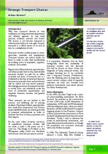
transport options available in the model for each Travel Zone will be realistic, specified as the key attributes of headway and journey time for each transit line. Detailing every transit service variation may also suggest a false level of STM precision. Using ‗patterns‘ provides effective representation of transit services for the strategic application context, with reduced computational load. The use of ‗patterns‘ simplifies the input of data, and analysis of results, but some detail is lost in the process. Generating representative routing, frequency and journey time details is required for STM mode choice and assignment operations, and to provide a consistent basis for use in other scenarios. One overview measure of ‗representativeness‘ is the profile of bus transit line average speeds. Approximately 86% of routes have a mean speed between 10 and 30 kmh in one set of transit lines. Figure 7 shows a steep nose and tapered tail profile. Plotted outliers are checked to see if sensible – a congested inner-city route or a country route mostly on highway will have very different speeds. Other scenarios are also compared to see if differences reflect changes applied to prior year transit lines. Figure 7 Bus transit line average speed profile Mean Bus Itinerary Speeds 700

No of Itineraries

600 500 400 300 200 100 0 < 10

10 - 20

20-30

30-40

40-50

50-60

60-70

70+

Speed Bands

Geographically, representativeness means bus routings are close to the ‗on-the ground' track of buses. This is delivered through adding nodes and links, the checking processes and because network nodes are registered to corresponding intersections across the GMA. Bus access is modelled from Travel Zone centroids, with multiple centroid connector links providing direct paths to the public transport network. These centroid connectors are positioned so whichever direction the travel is in, an appropriate path for the travellers is available. Also, at a higher level, the transit parameter settings and transit service data are included in the STM validation processes.

13

ATRF 2010 Proceedings

6.2 Route Variations Patterns are used to represent level of service and are derived from timetable data. Minor variations in time and route are simplified. This approach provides consistency, is easily adaptable for future years, and readily communicable. Variations in services on the ground are reflected in model inputs in different ways. Some services operate as ‗out- and back‘, or on a circular routing, back to their starting points. Alternate termini, for example ‗Route 4‘ services to Wollongong University in lieu of Wollongong CBD require a variation. Even if most of the route is common with route 4 different trips will be modelled – not only destination, but travel times, trip purposes etc. Also the route 610X from Castle Hill to the City has some peak period services starting earlier from Kellyville (~7km further). Another case is where services run ‗express‘, omitting stops on a well loaded part of the route. Some route variations may evolve into separate routes, disappear completely, or become additional ‗ordinary‘ services on the normal route. With five year steps between model years, changes in routes must be expected as infrastructure, travel behaviour data, and fares. Residential population and other land use inputs are also likely to have changes over a five year period.

7. Conclusion This paper has explained the processes used to extract and consolidate bus data from electronic timetable, itinerary transformations for input to STM and the methods used to seek anomalies and rectify errors found. Key elements of this approach to coding public transport services are:   

electronic actual timetables are used, minor bus route variations are consolidated, transit line anomalies are identified with heuristics.

The procedures described above aim to deliver consistent, representative, and sufficient bus service inputs, fit for strategic modelling purposes. The use of automated processes expedites updating timetable information but brings its own issues. Some issues to consider if applying similar approaches to other strategic transport models are outlined below.

7.1.1 Scale effects The GMA is a large and diverse area, so significance of simplifying bus services can vary. Two extra peak period buses will noticeably cut headways in an outer area, but are insignificant on the busy approaches to the Sydney CBD. The bus service selection criteria should consider the ―commuter‖ period applicable in outer areas, which may be earlier than standard definition. In areas with sparse services the public transport option may be more akin to a ‗coach‘ service than a ‗route bus‘ service .

7.1.2 Temporal factors The process used for selecting bus patterns is primarily for the ‗morning peak‘ Time of Day, with services included when their midpoint is between 7am and 9am. For some projects a different period may be more appropriate. For example a single peak hour for services arriving at regional city CBD, or a three hour period to study longer distance travellers.

14

ATRF 2010 Proceedings

The bus patterns apply the travel times published in the timetable. This inherently assumes the timetables represent accumulated operator experience of day to day variability due to traffic, weather and passenger loadings. It implies passengers apply their experience with the timetabled headways and journey times when applicable to their travel decision making.

7.1.3 Spatial factors The STM uses straight links, so distances can be slightly understated. The effects are minimised as nodes are registered to matching intersections, with a resolution level of metres. One network node may represent multiple bus stops, both for interchanges and generally across the network. In the strategic model zone-based context this is an effective approach, although additional nodes should be considered if major changes are made to the zoning system. Travel Zone sizes vary across the GMA, with small zones tending to have high activity levels and network density, for example CBDs. At the other end of the scale the largest zones have lower activity levels and sparse bus services, typically comprising ex-urban areas.

>

Disclaimer: responsibility for the views expressed in this paper rests with the authors alone. >

References AECOM Consult Inc 2008, Technical Report FSUTMS Transit Model Development Guide Blainey SP and Preston JM 2010, Modelling local rail demand in South Wales, Transportation Planning and Technology, 33: 1, 55 — 73 Canning S, MVA Consultancy 2007, Recommendations Summary -Term Commission for the Maintenance and Enhancement of the Transport Model for Scotland, Edinburgh Carlson M, Arup 2003, Network Validation with Enif, 12th European EMME/2 Users Conference , Basel Carlson M and Armstrong J, Arup Transportation Planning 2007, Workarounds in Public Transit Modelling with EMME and Perl, 21st International Emme Users' Conference, Toronto Data Management Group, University of Toronto 2004, EMME/2 GTA Network Coding Standard 2001 Integrated Road and Transit Network, Toronto Eash, R and Lupa, M Chicago Area Transportation Study 1997, Transit Network Coding and Skimming Procedures for the ‗Transit Rich‘ Northeastern Illinois Region, 12th Annual International EMME/2 Users‘ Group Conference, San Francisco FHWA 1997, Model Validation and Reasonableness Checking Manual, Travel Model Improvement Program, FHWA-EP-01-023, Federal Highway Administration (BartonAschman Associates, Inc and Cambridge Systematics, Inc), Washington DC Holyoak NM, Taylor MAP, Oxlad, LM and Gregory, J 2005, Development of a new strategic planning model for Adelaide, ATRF2005, Sydney INRO, 2010, Emme User's Guide, Montreal

15

ATRF 2010 Proceedings

Milthorpe F, Transport and Population Data Centre, 2004, Coding Transit Itineraries, 2nd Australian EMME/2 Users' Conference, Sydney Nielsen, OA Mandel, B and Ruffert, E, 2001, Generalised transportation-data format (GTF) data, model and machine interaction, European Transport Conference Association for European Transport, London NSW Transport & Infrastructure, accessed 18-10-2010

www.transport.nsw.gov.au/tdc/travel.html,

Sydney,

Transport Data Centre, 2009, 2007 Household Travel Survey Summary Report, 2009 Release, TDC, Sydney

16