APPENDIX G GIS ANALYSIS PROCEDURES Determining Pedestrian Accessibility ....................................................................... G-1 Creating Pedestrian Network-Based Polygons.......................................................... G-1 Building a Network to Support Pedestrian Paths....................................................... G-6 Calculating Population and Employment Density................................................... G-14
List of Figures Figure G1. Create a Network Dataset..................................................................... G-2 Figure G2. Network Dataset Wizard ................................ ................................ ...... G-2 Figure G3. Connectivity Policy.............................................................................. G-2 Figure G4. Elevation of Path Segments.................................................................. G-3 Figure G5. Network Dataset Turn Table ................................................................ G-3 Figure G6. Creating Network Impedances ............................................................. G-4 Figure G7. Impedance Evaluators................................ ................................ .......... G-4 Figure G8. Direction Settings ................................................................................ G-5 Figure G9. Summary of Network Settings ............................................................. G-5 Figure G10. Adding Pedestrian Paths ....................................................................... G-7 Figure G11. Calculate Locations .............................................................................. G-8 Figure G12. Create Service Area Layer .................................................................... G-9 Figure G13. Load Network Facilities...................................................................... G-10 Figure G14. Setting Service Area Parameters ................................ ......................... G-11 Figure G15. Service Area Polygon Settings............................................................ G-12 Figure G16. Generalized Service Area Polygons .................................................... G-13 Figure G17. Detailed Service Area Polygons.......................................................... G-13
Determining Pedestrian Accessibility Geographic buffers are commonly used to determine the characteristics of an area within close proximity to transit service, as well as a means to measure the pedestrian accessibility of an area. These buffers are typically defined by circle-shaped polygons which have a radius defined by the maximum distance a person is likely to walk for high capacity transit service. The more commonly used distances are quarter mile, half mile and one mile. Another method that has recently gained a lot of attention in the modeling and research communities involves the development of network-based polygons that are constructed from the actual pedestrian network for an area, as opposed to the “as-the-crow-flies” method that defines the circular-polygons. Because of this characteristic, the network-based approach can be used to provide a better understanding of the overall pedestrian accessibility of an area. For comparative purposes, MTC has used both circular and network-based polygons in its research to support the travel behavior models used by the agency. While both approaches have been used, we have found that the network-based approach is more appropriate for determining the demographic characteristics of an area, as well as to measure its pedestrian accessibility. The following section provides a detailed explanation of our approach to defining Pedestrian Network based polygons. Creating Pedestrian Network-Based Polygons Since the release of ESRI’s Network Analyst extension to ArcGIS 9.1, it is very easy to create network-based polygons using the extension’s “Find Service Area” tool. “Service areas” are polygon regions that encompass all accessible streets around a facility or facilities within a specified impedance. There are three steps involved in generating network service areas. The first and most crucial step involves building a Network Dataset. Typical components used in a network dataset include: Streets or paths represented as polylines, attributes that can be used to define path connectivity policies, street or path names, elevation of path segments, functional hierarchy of streets, as well as some form of network impedance such as segment length or estimated speed of travel. A necessary sub-step in building the Network Dataset is the modification of a regional street dataset to include network impedances or cost attributes that can be used to model the flow of pedestrian traffic. Network impedances determine which roads are accessible to vehicles as well as pedestrians, the speed or time it takes to traverse a particular segment, as well as the length or distance traveled along the segment. The second step involves locating the facilities or locations from which the service area boundaries will be generated. Facilities must be located within an acceptable distance from the network paths in order to generate the network-based polygons. The third step is to generate the network-based polygons based on user-defined parameters. Examples of these parameters are the network impedance, the direction of travel, if u-turns are permitted, and the type of polygon generated. The Network Analyst extension contains several tools to facilitate these three steps.
G-1
Step 1: Build the Network Dataset A TeleAtlas GIS street dataset is used as the foundation for the Network Dataset. The street dataset contains roadway segments for the nine-county Bay Area region with attributes describing characteristics of these streets. This dataset was modified to handle pedestrian travel. These dataset modifications are described following the eight steps used to create the Network Dataset. 1. The street dataset is placed in a feature dataset within a personal geodatabase. Using ArcCatalog, select the feature dataset that contains the streets feature class. Select the File menu option and choose--New and choose the Network Dataset option. See Figure G1. This will launch the New Network Dataset wizard, which will guide you through the options to build a network dataset. See Figure G2. Figure G1. Create a Network Dataset
Figure G2. Network Dataset Wizard
2. The Connectivity Policy for network paths is defined as “Endpoint” as all paths in the street dataset have endpoint vertices at junctions with other paths. Figure G3. Connectivity Policy
G-2
3. Elevation of path segments in the dataset is contained in the fields F_ZLEV and T_ZLEV. These are used to model connectivity when the endpoints of path segments have the same elevation value. Differing elevation values of an overpass and a road that have coincident endpoints would not allow connectivity in the Network Dataset. Figure G4. Elevation of Path Segments
4. The Network Dataset is prepared for future use of a turn table by modeling turns in the network using the “Global Turns” turn source. Figure G5. Network Dataset Turn Table
G-3
5. Network attributes are created for all network impedances that may be used in analyses, as well as for other properties of network elements such as hierarchy and one-way restrictions. Here network attributes are created for Distance (vehicular), Drivetime (vehicular), Pedestrian_Distance, and Pedestrian_Time. Figure G6. Creating Network Impedances
6. Each network attribute is mapped to an evaluator in the streets dataset that will provide values for the network attribute when the network dataset is built. In this image, the evaluator for the Pedestrian_Time network attribute is set to the fields FT_Ped and TF_Ped. Figure G7. Impedance Evaluators
G-4
7. Directions are not required to build service areas; therefore we do not need to configure the parameters for this option. Figure G8. Direction Settings
8. A summary of the Network Dataset settings is presented. Clicking Finish begins the process of building the Network Dataset. Figure G9. Summary of Network Settings
G-5
Building a Network to Support Pedestrian Paths The pedestrian network that MTC has constructed is based upon the TeleAtlas GIS roadway dataset for the nine-county Bay Area region. This database contains roadway segments for the entire region, and provides a rich set of attributes that can be used for routing and geocoding functionality. However this dataset is primarily used to route vehicles, not pedestrians. Therefore it was necessary to develop selection criteria that could be used to reclassify many of the TeleAtlas base map attributes to support the development of the pedestrian network. The TeleAtlas Basemap contains the following attributes that can be used to build a network: 1. Roadway Segment Lengths 2. Roadway Speed Tables (Note: These speeds do not reflect posted roadway speed limits, however they represent average speeds associated with the functional class codes developed by TeleAtlas) 3. Roadway Classification- Highway, Freeway, Local Roads, etc. 4. Arterial Classification- Used for developing network hierarchies 5. Segment Impedance- Used to determine the cost to travel the segment. The values are based upon the length of the segment and its speed value. 6. Navigational Direction- Used to control the allowable direction of travel 7. Segment End Elevation- Indicates the planar connectivity for each end of a segment Building upon the attribute model developed by TeleAtlas, we added three fields to the database that could be used to classify pedestrian paths, PED_DIST, FT_PED, and TF_PED. The two latter fields represent the segment time impedance for each direction of pedestrian travel along a specific network segment. If a value is calculated as –1, the network segment would not be traversable by a pedestrian. This feature of network path building gives us greater control over how we build our network. We used the TeleAtlas Roadway Speed attribute to select all roads with a speed that is less than or equal to 35 mph, excluding roads that have a functional classification that prohibit pedestrian traffic, e.g., Freeway, Highway, Expressway Ramps. The roadway network around many of the transit stations in our region contains several pedestrian only paths that are not included in the TeleAtlas database. Therefore in order to accurately portray the pedestrian paths around these transit stations, new geographic features were digitized and added to the TeleAtlas roadway network. These additional paths were digitized based upon AirPhoto USA aerial imagery as well as field observations. See Figure G10.
G-6
Figure G10. Adding Pedestrian Paths
Once we selected the path segments appropriate for pedestrian travel, we then calculated the time impedance based upon the following formula: Time Impedance = (Segment Length*Average Walking Speed) Segment Length is calculated in miles, and Average Walking Speed is calculated in miles per hour. For average walking speed, we used a value of 3 mph. Using the time impedance and Segment Length fields we could calculate service areas based upon time (duration) of travel, and distance of travel. For the purposes of this study we used distance of travel.
G-7
Step 2: Locate the Network Facilities After the Network Dataset is built, the facilities, or locations around which the service areas will be created, are located on the network. For this study, we used the existing rail and ferry station in the nine-county Bay Area region. In order to locate the existing transit stations as facilities on the pedestrian network, we first had to ensure that the station points were within a specified search tolerance of the pedestrian network. Once we were relatively sure that each station point was within this search tolerance, we used the Network Analyst tool “Calculate Locations” in ArcToolbox to define the location of the points on the pedestrian network. This process involves the following steps. 1. Select input point features for which locations will be calculated. 2. Choose the Network Dataset that will be used to calculate the locations. 3. Specify a search tolerance to be used when locating the facilities on the network paths. 4. Specify the search criteria that will be used when finding locations. This step allows the users to select the road classes that are only accessible to pedestrians. Figure G11. Calculate Locations
Step 3: Generate Service Area Buffers Once the Network Dataset is complete and the facility locations are calculated, the network-based polygons can be generated using these two files and ArcMap. The following steps describe this process. 1. The Network Dataset and facility feature layer are added to the ArcMap project and a Service Area Analysis Layer is created.
G-8
Figure G12. Create Service Area Layer
2. The facility features are loaded in the Network Analyst window by right-clicking Facilities and selecting Load Locations. A sort order can be applied to the list of facilities. The option to Use Network Location Fields is chosen in order to use the values previously calculated in Step 2.
G-9
Figure G13. Load Network Facilities
3. The parameters for the service areas are set in the Analysis Layer Properties window. The service area is calculated on the pedestrian distance impedance with default breaks at 0.25, 0.5, and 1 mile. The direction of travel is away from facility, U-Turns are allowed everywhere and there are no one-way restrictions on use of network paths.
G-10
Figure G14. Setting Service Area Parameters
G-11
4. In the Polygon Generation tab, further parameters are set for the analysis. Generalized service area polygons are selected with separate polygons for each facility and with an overlap type of rings. Figure G15. Service Area Polygon Settings
G-12
Generalized polygons were created in this analysis because less processing time is required and service areas were created for a large number of facilities. The resulting service areas are less accurate than if detailed polygons were created. Generalized polygons have more linear boundaries due to extrapolation between a small set of sample points representing the distance from the facility and may slightly exaggerate the pedestrian accessibility around a transit station. See Figure G16. Detailed polygons can have more elaborate boundaries as a greater number of sample points are generated. See Figure 17. Figure G16. Generalized Service Area Polygons Figure G17. Detailed Service Area Polygons
G-13
Calculating Population and Employment Density Problem Statement Using population, household and employment data by census tract from Projections 2005, estimate the total population, households and jobs in 2000 within a half-mile pedestrian buffer for existing rail station and ferry terminal locations in the nine-county bay area region. The size of a station buffer will typically include a single census tract, aggregations of multiple census tracts, and most often portions of multiple census tracts. In order to determine the population, household, and employment characteristics within a defined buffer distance of a station location using census tract data, a method had to be devised that considers the disparate spatial differences of census tracts and the pedestrian buffers. The following section describes the methodology used to calculate total population and jobs within the half-mile pedestrian network based buffers of existing rail and ferry terminal locations. Methodology An easy way to estimate the demographic characteristics of an area using data that represents two different geographic extents (Census Tracts and Existing Land Use) is to first identify a common unit of measurement that can be used to quantify the characteristics across the entire geographic area being studied. In this case, we used the areas density (population per acre/ households per acre/ employment per acre) as a common unit of measurement. The density of an area can easily be determined by dividing the total units of measurement, by the total land area for that given activity. We assume that all population and household activities occur only on lands identified in the Existing Land Use database for residential activity, and that employment activities occur only on land uses that support employment activities (Commercial, Industrial, etc.). In order to do this we first had to create a geographic intersection of the census tract polygon boundaries with the Existing Land Use based polygon boundaries. We only used the land use polygons associated with Residential or employment activities. We then calculated population density by dividing the total population within the defined census tract by the total land area (acres) within that census tract identified as residential land use, to determine the population per acre. Since we are trying to estimate totals for population, households and employment, for an area with a known, quantifiable area, we can use the density the entire area being studied. Since we are working with Using average density as a unit of measurement, a spatial model was developed using Geographic Information Systems (GIS) analysis methods, using ABAG’s Existing Land Use database in a process to disaggregate total population and households by census tract to residential supporting land uses, and total jobs by census tract to employment supporting land uses,. In order to disaggregate the total population and households by census tract G-14
This was accomplished by using the total population and households and population area (in square meters) of the polygon based land use data to calculate the population and household densities based upon the total population, households and employment of a given area, divided by the total area of residential and emplyIn order to estimate the totals for population, households and employment within each half-mile pedestrian network buffer, we created a value raster populated with the average density per square 10 meters of constructed from 10 meter raster grid cells that contain values with defines the average density for ranges were calculated based upon the total population and jobs by land use area as defined by the 2000 Existing Land Use database. This density is then converted into 10 meter grid cells that are used to produce zonal statistics based upon the half-mile pedestrian network buffers of rail stations and ferry terminals in the region. This method assumes a constant average density within each of the zones where population and employment supporting land uses have been identified. Average Density =
Total Population, Jobs and Households in each tract divided by gross acres of existing residential and employmentgenerating land uses
GIS Tools Used Using the ArcGIS Spatial Analyst Extension, we estimate total population, households and jobs using the Zonal Statistics as Table Tool. This tool summarizes the values of a raster within the zones of another dataset and reports the results to a table.1 The average density is then multiplied by the total area of the buffer distance to estimate total population and employment within a half-mile and quarter mile radius of existing rail stations and ferry terminals for the region.
1
ESRI ArcGIS Spatial Analyst Functional Reference: Zonal Based Analysis Tools.
G-15