An Analysis of the Price Elasticity of Demand for Household Appliances

Larry Dale and K. Sydny Fujita February 2008

Energy Analysis Department Environmental Energy Technologies Division Lawrence Berkeley National Laboratory University of California Berkeley, CA 94720

DISCLAIMER This document was prepared as an account of work sponsored by the United States Government. While this document is believed to contain correct information, neither the United States Government nor any agency thereof, nor The Regents of the University of California, nor any of their employees, makes any warranty, express or implied, or assumes any legal responsibility for the accuracy, completeness, or usefulness of any information, apparatus, product, or process disclosed, or represents that its use would not infringe privately owned rights. Reference herein to any specific commercial product, process, or service by its trade name, trademark, manufacturer, or otherwise, does not necessarily constitute or imply its endorsement, recommendation, or favoring by the United States Government or any agency thereof, or The Regents of the University of California. The views and opinions of authors expressed herein do not necessarily state or reflect those of the United States Government or any agency thereof or The Regents of the University of California.

This work was supported by the Assistant Secretary for Energy Efficiency and Renewable Energy of the U.S. Department of Energy under Contract No. DE-AC02-05CH11231.

TABLE OF CONTENTS 1.0

2.0

3.0

4.0

5.0

INTRODUCTION……………………………………………………………..1 1.1 Literature Review……………………………………………………...1 1.1.1 Price………………………………………………………….....1 1.1.2 Income……………………………………………………….....2 1.1.3 Appliance Efficiency and Discount Rates……………………2 VARIABLES DESCRIBING THE MARKET FOR REFRIGERATORS, CLOTHES WASHERS, AND DISHWASHERS……………………………3 2.1 Physical Household and Appliance Variables…………………….....3 2.2 Economic Variables…………………………………………………...3 REGRESSION ANALYSIS OF VARIABLES AFFECTING APPLIANCE SHIPMENTS…………………………………………………………………..5 3.1 Broad Trends……………………………………………………….....5 3.2 Model Specification…………………………………………………...7 3.3 Model Discussion……………………………………………………...7 ANALYSIS RESULTS……………………………………………………..…8 4.1 Individual Appliance Model…………………………………….…....8 4.2 Combined Appliance Model…………………………………….…....9 CONCLUSION……………………………………………………………......9

APPENDIX A. A.1 A.2

ADDITIONAL REGRESSION SPECIFICATIONS AND RESULTS…………………………………………….11 Lower Consumer Discount Rate…………………………………………....11 Disaggregated Variables……………………………………………….…....11

APPENDIX B.

DATA USED IN THIS ANALYSIS………….………….….13

REFERENCES……………………………………………………………………....15

i

LIST OF CHARTS Chart 2.1 Chart 3.1

Trends in Appliance Shipments, Housing Starts and Replacements....4 Residual Shipments and Appliance Price………………………………6

LIST OF TABLES Table 1.1 Table 1.2 Table 2.1 Table 2.2 Table 3.1 Table 3.2 Table 4.1 Table 4.2 Table A.1 Table A.2

Estimates of the Impact of Price, Income and Efficiency on Automobile and Appliance Sales………………………………………..2 Discount Rates……………………………………………………………3 Physical Household and Appliance Variables………………………….4 Economic Variables……………………………………………………...4 Simple Estimate of Total Price Elasticity of Demand………………….6 Tabular Estimation of Relative Price Elasticity of Demand…………..6 Individual Appliance Model Results……………………………………9 Combined Appliance Model Results……………………………………9 Combined and Individual Results, 20% Discount Rate……………...11 Disaggregated Regression Results, 37% Discount Rate……………...12

ii

1.0

INTRODUCTION

This article summarizes our study of the price elasticity of demand1 for home appliances, including refrigerators, clothes washers and dishwashers. In the context of increasingly stringent appliance standards, we are interested in what kind of impact the increased manufacturing costs caused by higher efficiency requirements will have on appliance sales. We chose to study this particular set of appliances because data for the elasticity calculation was more readily available for refrigerators, clothes washers, and dishwashers than for other appliances. We begin with a review of the existing economics literature describing the impact of economic variables on the sale of durable goods. We then describe the market for home appliances and changes in it over the past 20 years. We conclude with summary and interpretation of the results of our regression analysis and present estimates of the price elasticity of demand for the three appliances. 1.1

Literature Review

There are relatively few studies measuring the impact of price, income and efficiency on the sale of household appliances. In this section we provide a short review of this literature which suggests the likely importance of these variables. 1.1.1

Price

The goal of many of the studies covered in this review is to measure the impact of price on sales in a dynamic market. One study of the automobile market prior to 1970 finds the price elasticity of demand to decline over time. The author explains this as the result of buyers delaying purchases after a price increase but eventually making the purchase out of necessity (Table 1.1).2 A contrasting study of household white goods also prior to 1970, finds the elasticity of demand to increase over time as more price-conscious buyers enter the market.3 A recent analysis of refrigerator market survey data finds that consumer purchase probability decreases with survey asking price.4 Estimates of the price elasticity of demand for different brands of the same product tend to vary. A review of 41 studies of the impact of price on market share found the average brand price elasticity5 to be -1.75.6 The average estimate of price elasticity of demand reported in

1

Price elasticity is the percent change in shipments given a percent change in price. S. Hymens "Consumer Durable Spending: Explanation and Prediction” Brookings Papers on Economic Activity. 1971 3 P. Golder and G. Tellis, "Beyond Diffusion: An Affordability Model of the Growth of New Consumer Durables" Journal of Forecasting. 1998. 4 D. Revelt and K. Train, "Mixed Logit with Repeated Choices: Household's Choice of Appliance Efficiency Level." Review of Economics and Statistics. 1997 5 Brand price elasticity is the percent change in shipments given a percent change in price for a particular brand of appliance. Sales of a particular brand of appliance will be more sensitive to price changes than sales of appliances in general. 6 G. Tellis. "The Price Elasticity of Selective Demand: A Meta-Analysis of Econometric Models of Sales". Journal of Marketing Research. 1988. 2

iii

these studies is -0.33 in the appliance market and -0.47 in the combined automobile and appliance markets. 1.1.2

Income

Higher income households are more likely to own household appliances.7 The impact of income on appliance shipments is explored in two econometric studies of the automobile and appliance markets. 8 9 The average income elasticity of demand is 0.50 in the appliance study cited in the literature review; the average income elasticity is much larger in the automobile study. Table 1.1

Estimates of the Impact of Price, Income and Efficiency on Automobile and Appliance Sales Price Elasticity

Product

Income Elasticity

Brand Price Implicit Discount Elasticity Rate

1

Model

Data years

-1.07 3.08 Linear Regression, stock adjustment 1 Automobiles 1 -0.36 1.02 Linear Regression, stock adjustment 2 Automobiles 2 -0.14 0.26 Cobb-Douglas, diffusion 1947-1961 3 Cloths Dryers 2 6 -.37 0.45 Cobb-Douglas, diffusion 1946-1962 4 Room Air Conditioner 2 -0.42 0.79 Cobb-Douglas, diffusion 1947-1968 5 Dishwasher 3 -0.37 39% Logit probability, using survey data. 1997 6 Refrigerators 4 7 -1.76 Multiplicative regregression 7 Various 5 8 Room Air Conditioner -1.72 Non-linear diffusion 1949-1961 5 -1.32 Non-linear diffusion 1963-1970 9 Cloths Dryers Sources: 1 S. Hymens. "Consumer Durable Spending: Explanation and Prediction" Brookings Papers on Economic Activity. 1971 2 P. Golder and G. Tellis, "Beyond Diffusion: An Affordability Model of the Growth of New Consumer Durables" Journal of Forecasting. 1998. 3 D. Revelt; K.Train,"Mixed Logit with Repeated Choices: Households Choice of Appliance Efficiency Level" Review of Economics and Statistics. 1997 4 G. Tellis. "The Price Elasticity of Selective Demand: A Meta-Analysis of Econometric Models of Sales". Journal of Marketing Research. 1988. 5 D.Jain; R.Rao. "Effect of Price on the Demand for Durables: Modeling, Estimation and Findings" Journal of Business and Economic Statistics. 1990.

Time Period Short run Long run Mixed Mixed Mixed Short run Mixed Short run Short run

Notes: 6 Logit probability results are not directly comparable to other elasticity estimates in this table. 7 Average brand price elasticity across 41 studies.

1.1.3

Appliance Efficiency and Discount Rates

Many studies estimate the impact of appliance efficiency on consumer appliance choice. Typically, this impact is summarized by the implicit discount rate, i.e., the rate consumers use to compare future appliance operating cost savings against an appliance purchase price premium. One early and much cited study concludes that consumers use a 20% implicit discount rate when purchasing room air conditioners (Table 1.2).10 A survey of several studies of different appliances suggests that the average consumer implicit discount rate is about 37%.11 In Section 3, we use a discount rate of 37% to estimate

7

Energy Information Agency. “The Effect of Income on Appliances in U.S. Households.” U.S. Department of Energy: http://www.eia.doe.gov/emeu/recs/appliances/appliances.html. 2002. Accessed February 1, 2007 8 S. Hymens "Consumer Durable Spending: Explanation and Prediction." Brookings Papers on Economic Activity. 1971 9 P. Golder and G. Tellis, "Beyond Diffusion: An Affordability Model of the Growth of New Consumer Durables" Journal of Forecasting. 1998. 10 J. Hausman. "Individual discount rates and the purchase and utilization of energy using durables." The Bell Journal of Economics. 1979. 11 K. Train. "Discount rates in consumer' energy related decisions: a review of the literature." Energy. 1985

2

discounted operating costs, based on appliance efficiency. The implications of a 20% discount rate are considered in Appendix A. Table 1.2

Discount Rates Implicit Discount Rate

Product 1

Room Air Conditioners 2 Household Appliances

Model

20% 3 37%

Qualitative choice, survey data Assorted 1 J. Hausman. "Individual discount rates and the purchase and utilization of energy using durables."

The Bell Journal of Economics. 1979. 2 K. Train. "Discount rates in consumer' energy related decisions: a review of the literature." Energy. 1985 3 Averaged across several household appliance studies referenced in this work.

2.0

VARIABLES DESCRIBING THE MARKET FOR REFRIGERATORS, CLOTHES WASHERS, AND DISHWASHERS

In this section we evaluate variables that appear to account for refrigerator, clothes washer and dishwasher shipments, including physical variables and economic variables. 2.1

Physical Household and Appliance Variables

Several variables influence the sale of refrigerators, clothes washers and dishwashers. The most important for explaining appliance sales trends are the annual number of new households formed (housing starts) and the number of appliances reaching the end of their operating life (replacements). Housing starts influence sales because new homes are often provided with – or soon receive – new appliances, including dishwashers and refrigerators. Replacements are correlated with sales because new appliances are typically purchased when old ones wear out. In principle, if households maintain a fixed number of appliances, shipments should equal housing starts plus appliance replacements.

2.2

Economic variables

Appliance price, appliance operating cost and household income are important economic variables affecting shipments. Low prices and operating costs encourage household appliance purchases and a rise in income increases householder ability to purchase appliances. In principle, changes in economic variables should explain changes in the number of appliances per household. During the 1980 – 2002 study period, annual shipments grew 69% for clothes washers, 81% for refrigerators and 105% for dishwashers (Table 2.1). This rising shipments trend is explained in part by housing starts, which increased 6% and by appliance replacements, which rose between 49% and 90% over the period (Table 2.1).12 For 12

Appliance replacements are determined from the expected operating life of refrigerators (19 years), cloths washers (14 years) and dishwashers (12 years) and from past shipments. Replacements are further described in Appendix II.

3

mature markets such as these, replacements exceed appliance sales associated with new housing construction. Table 2.1

Physical Household and Appliance Variables

Appliance Refrigerators Clothes Washers Dishwashers

1980 5.124 4.426 2.738

Shipments 2002 9.264 7.492 5.605

Housing Starts 1980 2002 1.723 1.822 1.723 1.822 1.723 1.822

Change (%) 81% 69% 105%

Replacements 1980 2002 3.93 5.84 3.66 5.50 1.99 3.79

Change (%) 6% 6% 6%

Change (%) 49% 50% 90%

Shipments: Number of units sold, in millions. AHAM Factbook and Appliance Magazine. Housing starts: Annual number of new homes constructed. U. S. Census. Replacements: Average of annual lagged shipments, with lag equal to expected appliance operating life, plus or minus 5 years.

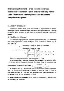
Nevertheless, it is apparent that appliance shipments increased somewhat more rapidly than housing starts and replacements. This is shown by comparing the beginning and end points of lines representing “starts plus replacements” (uppermost solid line) and “shipments” (diamond linked line) (Chart 2.1). In 1980 the “shipment” line begins below the “starts plus replacements” line. In 2002, the “shipments” line ends above the “starts plus replacements” line. This more rapid increase in shipments, compared to housing starts plus replacements, suggests that the appliance per household ratio increased over the study period. Chart 2.1

Trends in Appliance Shipment, Housing Starts and Replacements

Refrigerator Shipments

8

10 9

Dishwasher Shipments 6

New Housing 7

Retirements 8

Clothes Washer Shipments

5

Shipments

6 4

5

6

Millions .

Millions .

Millions .

7

4

5 4

3

3 2

3

2 2

0

1980

1

1

1

0

1984

1988

1992

1996

2000

1980

0

1984

1988

1992

1996

2000

1980

1984

1988

1992

1996

2000

Economic variables, including price, cost and income, may explain this increase in appliances per household. Over the period, appliance prices increased 40% to 50%, operating costs fell between 33% and 72% and median household income rose 16% (Table 2.2). Table 2.2

Economic Variables

Appliance Refrigerators Clothes Washers Dishwashers

Price 1980 1208 779 713

2002 726 392 368

Change (%) -40% -50% -48%

Operating Cost 1980 2002 333 94 262 175 183 95

Change (%) -72% -33% -48%

Household Income 1980 2002 37,447 43,381 37447 43381 37447 43381

Price. Shipment weighted retail sales price, in 1999 dollars for selected years. AHAM Fact Book, TSDs. Operating cost. Annual electricity price times electricity consumption (UEC), for selected years. 1999 dollars. AHAM fact book. Income. Mean household income. U.S. Census.

4

Change (%) 16% 16% 16%

3.0

REGRESSION ANALYSIS OF VARIABLES AFFECTING APPLIANCE SHIPMENTS

Little data is available for estimating the impact of economic variables on the demand for appliances. Industry operating cost data is incomplete – appliance energy use data is available for only 12 years of the 1980-2002 study period. Industry price data is also incomplete – available for only 8 years of the study period for each of the appliances. The lack of data suggests that regression analysis can at best evaluate broad data trends, utilizing relatively few explanatory variables. In this section we begin by describing broad trends apparent in the economic and physical household data sets. We then specify a simple regression model to measure these trends, making assumptions to minimize the number of explanatory variables. Finally, we present results of the regression analysis and our estimate of the price elasticity of demand for appliances. In an appendix, we also present the results of regression analysis performed with more complex models, and used to test assumptions made to specify the simple model. These results support the simple model specification, and estimates of the price elasticity of appliance demand measured with that model.

3.1

Broad Trends

In this section we review trends in the physical household and economic data sets and posit a simple approach for estimating the price elasticity of appliance demand. As noted above, the physical household variables (starts and appliance replacements) explain most of the variability in appliance shipments over the period.13 We assume the rest of the variability in shipments (residual shipments) is explained by economic variables, and present a tabular method for measuring price elasticities described below. To illustrate this tabular approach, we define two new variables – residual shipments and total price. Residual shipments are defined as the difference between shipments and physical household demand (starts plus replacements). Total price is defined as appliance price plus the present value of lifetime appliance operating cost.14 Over the study period, residual shipments increase 30% for refrigerators, 19% for clothes washers and 23% for dishwashers in proportion to total shipments. At the same time, total prices decline 47%, 45% and 48% for refrigerators, clothes washers and dishwashers, respectively. Assuming that total price explains the entire change in per household appliance purchases, we calculate a rough estimate of the total price elasticity of demand equal to -.48 for refrigerators, -.32 for clothes washers and -.37 for dishwashers (Table 3.1). 13

A log linear regression of the form: Shipments = a + b (Housing starts) + c (Retirements), indicates that these two variables explain 89% of the variation in refrigerator shipments, 97% of the variation in cloths washer shipments and 97% of the variation in dishwasher shipments. 14 Present value operating cost is calculated assuming a 19 year operating life for refrigerators, 14 year operating life for washing machines and a 12 year operating life for dishwashers. A 37% discount rate is used to sum annual operating costs into a total present value operating cost.

5

Table 3.1

Simple Estimate of Total Price Elasticity of Demand

Appliance Refrigerators Clothes Washers Dishwashers

Residual Shipments, millions 2002 2.1 1.1 1.0

Residual Shipments, millions 1980 2002 -0.5 1.6 -1.0 0.2 -1.0 -0.01

Change (%) 30% 19% 23%

Change (%) -61% -59% -64%

Total Price 1980 2002 1541 820 1042 567 896 464

Elasticity -0.48 -0.32 -0.37

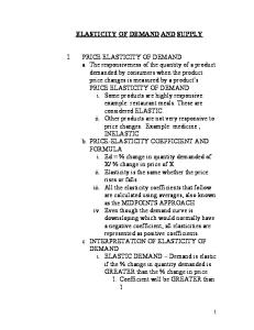
The negative correlation between total price and residual shipments suggested by these negative price elasticities is illustrated in a graph of residual shipments and total price (Chart 3.1).

Residual Shipments and Appliance Price Refrigerators

Residual Shipments

1200

800

-1.0

0.0

1.0

2.0

1000

.

. Residual Shipments

1600

400 -2.0

1200

Interpolation Observation

Dishwashers

.

2000

Clothes Washers

Residual Shipments

Chart 3.1

1000

800

600

400 -1.5

Total Price

-1.0

-0.5

0.0

0.5

800

600

400

200 -2.0

Total Price

-1.5

-1.0

-0.5

0.0

0.5

Total Price

Household income rose during the study period, making it easier for households to purchase appliances. Assuming that a rise in income has a similar impact on shipments as a decline in price, we incorporate the impact of income by defining a third variable, termed relative total price, calculated as total price divided by household income.15 The percent decline in relative price for the three appliances divided by the percent change in residual shipments suggests a rough estimate of relative price elasticity equal to -.40 for refrigerators, -.26 for clothes washers and -.30 for dishwashers (Table 3.2). Table 3.2 Appliance Refrigerators Clothes Washers Dishwashers

Tabular Estimation of Relative Price Elasticity of Demand Residual Shipments 1980 2002 -0.532 1.597 -0.953 0.174 -0.974 -0.005

Change (%) 30% 19% 23%

15

Relative Total Price 1980 2002 0.041 0.019 0.028 0.013 0.024 0.011

Change (%) -74% -72% -76%

Elasticity -0.40 -0.26 -0.30

Recall that the income elasticity of demand cited in the literature review is .50 and the price elasticity of demand cited in the review averages -.35. This suggests that combining the effects of income and price will yield an elasticity less negative than price elasticity alone.

6

3.2

Model Specification

The limited price data suggests using a simple regression model to estimate the impact of economic variables on shipments, using few explanatory variables. The equation chosen for this analysis includes one physical household variable (starts plus replacements) and one relative price variable (the sum of price plus operating cost, divided by income) (Equation 3.1). These variables in this model, termed the individual appliance model, are defined in foot notes below and in Appendix B. 16 17 Equation 3.1 Shipments = a + b (Relative Price) + c (Starts+Replacements) The natural logs are taken of all variables so that the estimated coefficients for each variable in the model may be interpreted as the percent change in shipments associated with the percent change in the variable. Thus, the coefficient b in this model is interpreted as the relative price elasticity of demand for the three appliances. A combined regression equation is used to estimate an average price elasticity of demand across the three appliances, using pooled data in a single regression (Equation 3.2). A combined regression specification is justified, given limited data availability and similarity in price and shipment behavior across appliances (Chart 3.1). Thus, the model represented by the combined regression equation is considered the basic model in our analysis of appliance shipments. Equation 3.2 Shipments = a + b (Relative Price) + c (Starts+Replacements) + d (CW) + e (DW)18 3.3

Model Discussion

The most important assumption used to specify this model is that changes in economic variables over the study period – income, price and operating cost – are responsible for all observed growth in residual appliance shipments. In other words, we assume other possible explanations, such as changing consumer preferences and increases in the quality of appliances, had no impact. This assumption seems unlikely but without additional data, the impact of this assumption on the price elasticity of demand cannot be measured. We effectively assume that changes in consumer preferences and appliance characteristics, while affecting which specific models are purchased, have relatively little impact on the total number of appliances purchased in a year. Three additional assumptions used to specify this model deserve comment. The relative price variable is specified in the model, assuming that (1) the correct implicit discount 16

Shipments is the quantity of appliances sold, housing starts is the number of new homes, replacements is the number at the end of their operating life and ability to pay is defined in footnote (15) below (natural logs taken of all variables). 17

Relative Price = 18

Total Price (First Price) + (Present Value Operating Cost) . = Income Income

CW and DW are dummy variables for clothes washers and dishwashers.

7

rate is used to combine appliance price and operating cost and that (2) rising income has the same impact on shipments as falling total price. The starts + replacements variable is specified, assuming (3) that starts and replacements have similar impacts on shipments. To investigate the first assumption about discount rates, we calculated “present value operating cost” using a 20% implicit discount rate and performed a second regression analysis of equation 1. The results of this analysis, presented in Appendix A, indicate that the elasticity of relative price is relatively insensitive to changes in the discount rate. To investigate the second and third assumptions, we specified a regression model separating income from total price and replacements from starts, thus adding two additional explanatory variables to the basic model (Equation 3.3). Equation 3.3 Shipments = a + b (Total Price) + c (Income) + d (Starts) + e (Replacements) + f (CW) + g (DW). The results of the regression analysis of this model are also presented in Appendix A. These results suggest that the elasticity of total price (coefficient b) is relatively insensitive to changes in the treatment of income and starts + replacements in the model.

4.0

ANALYSIS RESULTS

4.1

Individual Appliance Model

The individual appliance regression equations are specified as described in equation 3.1. In regression analysis of this model, the elasticity of relative price (b) is estimated to be 0.4 for refrigerators, -0.31 for clothes washers and -0.32 for dishwashers (Table 6), averaging -0.35. These elasticities are similar to those reported in the literature survey for appliances (Table 1.1). They are remarkably similar to the price elasticity calculated using a tabular approach presented above (Table 3.2). The estimated coefficient associated with the starts + replacements variable is close to one. A coefficient equal to one for this variable would imply that shipments increase in direct proportion to an increase in starts + replacements, holding economic variables constant. The high R-squared values (above 95) and t-statistics (above 5) in the results provide a measure of confidence in this analysis, despite the very small data set. Table 4.1

Individual Appliance Model Results

Variable Intercept Relative Full Price Starts+Replacements 2

R Observations

Refrigerator Coefficient tStat -1.51 -7.26 -0.40 -6.60 1.05 5.90

Clothes Washer Coefficient tStat -1.47 -8.23 -0.31 -5.69 1.08 6.41

Dishwasher Coefficient tStat -2.08 -16.78 -0.32 -7.03 1.35 11.46

0.954 23

0.954 23

0.975 23.00

8

4.2

Combined Appliance Model

The combined appliance regression equation is specified as described in equation 3.2. Our regression analysis indicates that the model fits the existing shipments data well (high R-squared) and that the variables included in the model are statistically significant (Table 4.2). The elasticity of relative price estimated with this model is -0.34, close to the average value estimated in the individual appliance models (-0.35). It is also similar to elasticity estimates reported in the literature survey and calculated using the tabular approach above. Table 4.2

Combined Appliance Model Result

Variable Intercept Relative Full Price Starts+Replacements CW DW R2 Observations

5.0

Coefficient -1.60 -0.34 1.21 -0.20 -0.32

tStat -15.54 -10.74 13.95 -9.04 -6.58 0.983 69

CONCLUSION

At the beginning of this report, we describe the results of a literature search, tabular analysis and regression analysis of the impact of price and other variables on appliance shipments. In the literature, we find only a few studies of appliance markets that are relevant to this analysis, and no studies using time series price and shipments data after 1980. The information that can be summarized from the literature, suggests that the demand for appliances is price inelastic. Other information in the literature suggests that appliances are a normal good, such that rising incomes increase the demand for appliances. Finally, the literature suggests that consumers use relatively high implicit discount rates, when comparing appliance prices and appliance operating costs. There is not enough price and operating cost data available to perform complex analysis of dynamic changes in the appliance market. In this analysis, we use data available for refrigerators, clothes washers and dishwashers to evaluate broad market trends and to perform simple regression analysis. These data indicate that there has been a rise in appliance shipments and a decline in appliance price and operating cost over the period. Household income has also risen during this time. To simplify the analysis, we combined the available economic information into one variable, termed relative price, and used this variable in a tabular analysis of market trends, and a regression analysis.

9

Our tabular analysis of trends in the number of appliances per household suggests that the price elasticity of demand for the three appliances is inelastic. Our regression analysis of these same variables suggests that the price elasticity of demand is -.35, averaged over the three appliances. The price elasticity is similar to estimates in the literature. Nevertheless, we stress that the measure is based on a small data set, using very simple statistical analysis. More important, the measure is based on an assumption that economic variables, including price, income and operating costs, explain most of the trend in appliances per household in the United States since 1980. Changes in appliance quality and consumer preferences may have occurred during this period, but they are not accounted for in this analysis. The capacity of most appliances has increased since 1980, and it is likely that there have been increases in quality and durability as well. If these factors have impacted the sales of appliances, our estimate of the price elasticity of demand is an over-estimate, since some of the increases in sales over the 1980-2002 time period would have been driven by changing preferences rather than decreasing prices.

10

APPENDIX A.

ADDITIONAL REGRESSION SPECIFICATIONS AND RESULTS

As mentioned above, the implicit price variable in the basic regression model is specified using a 37% implicit discount rate, to aggregate appliance price and operating cost. In addition, the implicit price variable is defined assuming that rising income has the same impact on shipments as falling total price. Similarly, the Starts+Replacements variable is defined assuming that housing starts have a similar impact on shipments as appliance replacements. A.1

Lower Consumer Discount Rate

To investigate the first assumption about discount rates, we calculated “present value operating cost” using a 20% implicit discount rate and performed a second regression analysis of equations 3.1 and 3.2. The estimated coefficient associated with the relative price variable in these regressions is almost identical to the coefficients estimated for same variable reported above using a 37% implicit discount rate. The elasticity of relative price calculated using a 20% discount rate is -.33 in the combined regression and averages -.35 for the three appliances (Table A.1). The elasticity of price calculated using a 37% discount rate is -.34 in the combined regression and averages -.35 for the three appliances. We conclude from this analysis that the elasticity of relative price is relatively insensitive to changes in the discount rate. Table A.1 Combined and Individual Results, 20% discount rate Variable Intercept Relative Full Price Starts+Replacements CW DW

Coefficient -1.53 -0.33 1.20 -0.18 -0.32

R2 Observations Variable Intercept Relative Full Price Starts+Replacements

0.982 69 Refrigerator Coefficient tStat -1.36 -6.26 -0.38 -6.50 1.04 5.73

Clothes Washer Coefficient tStat -1.41 -7.49 -0.32 -5.29 1.06 5.83

Dishwasher Coefficient tStat -2.04 -17.23 -0.33 -7.30 1.34 11.64

0.953 23

0.950 23

0.977 23.00

R2 Observations

A.2

tStat -14.61 -10.69 13.65 -8.69 -6.57

Disaggregated Variables

To investigate the second and third assumptions, we constructed a regression model separating income from total price and replacements from starts, thus adding two additional explanatory variables to the basic model (Equation A.1). Equation A.1 Shipments = a + b (Total Price) + c (Income) + d (Starts) + e (Replacements) + f (CW) + g (DW). The estimated coefficient associated with the total price variable in these regressions is almost identical to the coefficients estimated for the relative price variable reported above. The elasticity

11

of total price in Equation A.1 is -.36 in the combined appliance regression and averages -.35 for the three appliances (Table A.2). The elasticity of relative price in Equation 3.2 is -.34 in the combined regression and averages -.35 across the individual appliances (Tables 4.1 and 4.2). We conclude that the price elasticity calculated in this analysis is relatively insensitive to the specification of household income and starts + replacements variables in the model.

Table A.2

Disaggregated Regression Results, 37% Discount Rate

Variable Intercept Income Full Price Houseing Starts Replacements CW DW R2 Observations Variable Intercept Income Full Price Houseing Starts Replacements R2 Observations

Coefficient -2.92 0.58 -0.36 0.44 0.62 -0.24 -0.46

tStat -1.26 2.92 -7.06 10.02 8.12 -9.25 -7.68 0.985 69

Refrigerator Coefficient tStat -6.19 -2.24 0.89 3.80 -0.35 -5.48 0.41 7.38 0.56 6.06

Clothes Washer Coefficient tStat -6.64 -1.63 0.87 2.31 -0.27 -2.51 0.25 3.29 0.56 2.09

Dishwasher Coefficient tStat 1.00 0.23 0.20 0.52 -0.43 -5.18 0.62 8.24 0.65 5.86

0.984 23

0.958 23

0.979 23

12

APPENDIX B.

DATA USED IN THIS ANALYSIS

1. Appliance Shipments: Shipments are defined as the annual number of units shipped in millions. These data were collected from the Association of Home Appliance Manufacturers (AHAM) and Appliance Magazine as annual values for each year, 1980-2002. 2. Appliance Price: Price is defined as the shipments weighted retail sales price of the unit in 1999 dollars. Price values for 1980, 1985, 1986, 1991, 1993, 1994, 1998, and 2002 were collected from The AHAM. Fact Book and Department of Energy Technical Support Documents. Price values for other years were interpolated from these eight years of data. 3. Housing Starts: Housing starts data were collected from U.S. Census construction statistics (C25 reports) as annual values for each year, 1980-2002. 4. Replacements: Retirement-driven replacements are estimated with the assumption that some fraction of sales arise from consumers replacing equipment at the end of its useful life. Since each appliance has a different expected lifespan (19 years for refrigerators19, 14 years for clothes washers20, 12 years for dishwashers21), replacements are calculated differently for each appliance type. Replacements are estimated as the average of shipments 14-24 years previous for refrigerators, 9-19 years previous for clothes washers, and 7 to 17 years previous for dishwashers. Historical shipments data were collected from AHAM and Appliance Magazine. 5. Annual Electricity Consumption: Electricity Use (UEC) is defined as the energy consumption of the unit in kilowatt-hours. Electricity consumption is dependent on appliance capacity and efficiency. These data were provided by AHAM for 1980, 1990-1997 and 1999-2002. Data were interpolated in the years for which data were not available. 6. Operating Cost: Operating Cost is the present value of the electricity consumption of an appliance over its expected lifespan. The life spans of refrigerators, clothes washers and dishwashers are assumed to be 19, 14, and 12 years respectively. Discount rates of 20%22 and 37%23 were used, producing similar estimates of price elasticity. A study by Hausman 19

Duemling, Reubin. 1999 “Product Life of Refrigerators.” University of California, Berkeley, Energy and Resources Group masters thesis. 20 U.S. Department of Energy. 2000. “Technical Support Document (TSD): Energy Efficiency Standards for Consumer Products: Clothes Washers.” 21 U.S. Department of Energy. “Technical Support Document: Home Appliances.” 22 Hausman, Jerry A. 1979 “Individual discount rates and the purchase and utilization of energy-using durables.” 23 Train, Kenneth E. and Terry Atherton. 1995 The Energy Journal, “Rebates, loans, and customers’ choice of appliance efficiency level: combining stated- and revealed-preference data.”

13

recommended a discount rate of “about 20%” in its introduction, and presented results ranging from 24.1% to 29% based on his calculations for room air conditioners. A study by Train suggests a range of implicit discount rates averaging 35% for appliances. 7. Income: Median annual household income in 2003 dollars. This data was collected for each year, 1980-2002, from Table H-6 of the U.S. Census, http://www.census.gov/hhes/income/histinc/h06ar.html (accessed February 1, 2007).

14

REFERENCES Association of Home Appliance Manufacturers. Fact Book. 2003. Duemling, R. Product Life of Refrigerators. University of California, Berkeley, Energy and Resources Group Master’s Thesis. 1999. Energy Information Agency. The Effect of Income on Appliances in U.S. Households. U.S. Department of Energy. 2002. Golder, P. and G. Tellis. Beyond Diffusion: An Affordability Model of Growth of New Consumer Durables. Journal of Forecasting. 1998. Hausman, J. Individual Discount Rates and the Purchase and Utilization of Energy Using Durables. The Bell Journal of Economics. 1979. Hymens, S. Consumer Durable Spending: Explanation and Prediction. Brookings Papers on Economic Activity. 1971. Jain, D. and R. Rao. Effect of Price on the Demand for Durables: Modeling, Estimation and Findings. Journal of Business and Economic Statistics. 1990. Revelt, D. and K. Train. Mixed Logit with Repeated Choices: Household’s Choice of Appliance Efficiency Level. Review of Economics and Statistics. 1997 Tellis, G. The Price Elasticity of Selective Demand: A Meta-Analysis of Econometric Models of Sales. Journal of Marketing Research. 1998. Train, K. Discount Rates in Consumer Energy Related Decisions: a Review of the Literature. Energy. 1985. Train, K. and T. Atherton. Rebates, Loans, and Customers’ Choice of Appliance Efficiency Level: Combining Stated- and Revealed-Preference Data. The Energy Journal. 1995.

15