The yen/dollar exchange rate in 1998: views from options markets By Neil Cooper and James Talbot of the Bank’s Monetary Instruments and Markets Division.(1) 1998 was a period of unprecedented volatility for the yen/dollar exchange rate. To help to assess market participants’ views on exchange rate developments, the Bank of England uses a range of techniques that employ information from the over-the-counter (OTC) currency options markets. This article describes these techniques and shows how they can be used to assist our understanding of market perceptions of the yen/dollar exchange rate over this period. Introduction The exchange rate for the Japanese yen against the US dollar fluctuated widely during 1998, as shown in Chart 1. The yen depreciated from ¥131 on 1 January to ¥147 on 11 August, an eight-year low against the dollar.(2) But it then appreciated by 14% on 6–8 October, reaching ¥111. The yen/dollar rate ended the year at ¥114 intraday. Chart 1 Yen vs dollar exchange rate during 1998 Yen/dollar
Japanese government announced the largest-ever fiscal package, comprising ¥12 trillion of spending and ¥4 trillion of tax cuts. This was followed by intervention by the Bank of Japan later in the day. On 10 April, a bank holiday for most Western markets, the Bank of Japan intervened again; the yen appreciated against the dollar from ¥132 to ¥128 during Tokyo trading, but fell back over the next few days to its pre-intervention level. The second major intervention to support the yen was conducted in conjunction with the US Federal Reserve on 17 June. The yen appreciated from ¥143 to ¥137 on the day, but by 25 June was back at ¥142.
150 145 140 135 130 125
This article describes the techniques used by the Bank of England to extract information from foreign exchange options traded on the over-the-counter (OTC) market. It also demonstrates how information from these options can be used to investigate market views, addressing a number of questions of interest to central banks and other policy-makers, including:
120
●
did options markets predict the possibility of any of these dramatic movements in yen/dollar?
●
following the large shifts in the exchange rate, was volatility expected to persist?
●
did the correlation between movements in the dollar and the yen change substantially over the year?
●
were the intervention episodes successful in changing market views about the short-run path of the yen/dollar exchange rate?
115
J
F
M
A
M
J J 1998
A
S
O
N
D
110
The appreciation of the Japanese yen on 6–8 October was its largest two-day move since it began to float in February 1973, as a result of the collapse of the Bretton Woods agreement. Prior to this appreciation, US interest rate expectations had been declining since the Federal Reserve’s interest rate cut on 29 September: the March 1999 three-month eurodollar futures contract suggested that investors were expecting a further fall of 50 basis points before expiry. As the yen began to appreciate, the unwinding of large yen ‘carry trades’(3) exacerbated its rise. Some market comment at the time suggested that the moves were not expected to persist. We describe below what we can infer from derivatives markets about these expectations. There were also two major interventions by the monetary authorities to support the yen in 1998. On 9 April, the
Extracting information from options prices A wide range of financial instruments can be employed to infer market expectations of future levels of interest rates, exchange rates, inflation rates and commodity prices. But though assets, such as bonds and futures, can be used to extract point estimates for the expected future values of these variables, option prices can provide us with a
(1) Andy Bowen provided excellent programming assistance. (2) The market convention for quoting the yen/dollar exchange rate is in terms of the number of yen per dollar. Thus an increase in the exchange rate represents a depreciation (appreciation) of the yen (dollar). (3) A ‘carry trade’ is where an investor borrows money in yen at low Japanese interest rates and then invests this money in dollars at a higher interest rate; it is possible to make large profits if the yen does not appreciate.
68
The yen/dollar exchange rate in 1998: views from options markets
fuller picture of how the market views their future evolution. The most common and straightforward use of option prices is the calculation of implied volatility via the classic Black-Scholes (1973) model. Implied volatility is a measure of the degree of uncertainty that the market attaches to the returns on an asset. It is also possible to estimate the complete probability distribution for the future price of an asset and, for exchange rates, to calculate implied correlations between currencies.(1) All three of these measures are now used regularly by the Bank of England to analyse currency movements.
corresponds to the standard deviation of annualised returns. In fact, within the OTC foreign exchange options market, dealers typically give a quote in terms of implied volatility. Both participants to a trade know that to calculate the cash price, they apply this volatility to the Black-Scholes formula. This enables options traders to compare prices offered by different market-makers at different points in time without having to worry about changes in the underlying spot exchange rate affecting the quote. These implied volatility quotes are readily available from market-makers’ screens, on services such as Bloomberg and Reuters.(6)
Much of the Bank’s work on extracting information from options has focused on price information from the exchange-traded markets, particularly from the London International Financial Futures and Options Exchange (LIFFE). For foreign exchange options, however, liquidity is highest on the interbank or OTC markets. According to the recent triennial survey of foreign exchange and derivatives markets conducted by the Bank for International Settlements,(2) the average daily turnover of currency options on the OTC market was $87 billion worldwide, compared with an average daily turnover on the exchanges throughout the second quarter of 1998 of only $1.9 billion.(3) The main advantage of using OTC market data is the greater liquidity of the market; it also provides quotes on a wider range of exchange rates. But the OTC market has different ways of quoting prices, which require different methods for extracting information such as implied distributions.
Implied volatility is a measure of the uncertainty that the market attaches to future movements in the exchange rate over the remaining life of the option. By constructing a time series of implied volatility quotes, it is possible to track this uncertainty over time. Chart 2 shows one and twelve-month implied volatility for yen/dollar. Short-run uncertainty had been rising since the start of 1997, and increased further with the onset of the Asia crisis. But the unprecedented appreciation of the yen in early October triggered an even larger increase: one-month implied volatility reached 41%—more than double the previous high—following the move. Was this volatility anticipated in options markets? And was it expected to persist? Chart 2 Yen/dollar implied volatility Per cent One-month volatility
Deriving measures of uncertainty
39 34
In the Black-Scholes model, European-style currency options prices are determined by: (4)
44
(5)
29 24
●
the current spot rate;
●
domestic and foreign interest rates;
19 14 Twelve-month volatility
● ● ●
9
the maturity of the option; the strike price of the option; and the volatility of the underlying exchange rate.
Except for the volatility of the exchange rate, all of these variables are directly observable. Hence, for any given option price, it is possible to calculate the volatility implied by the Black-Scholes formula. This concept of implied volatility is widely used within options markets, and
J F M A M J J A S O N D J F M A M J J A S O N D 1997
4 0
98
By examining the implied volatilities of options for a range of maturities, it is possible to calculate forward volatility curves. These indicate how the market expects short-term volatility to change over each period of time, and allow us to examine issues such as whether volatility is expected to persist following a particularly turbulent time in the markets.(7) Chart 3 shows a time series of historical
(1) For more details on how implied probability density functions and implied exchange rate correlations are used by monetary policy-makers, see Bahra, B ‘Probability distributions of future asset prices implied by option prices’ Bank of England Quarterly Bulletin, August 1996, pages 299–311, and Butler, C and Cooper, N ‘Implied exchange rate correlations and market perceptions of European Monetary Union’, Bank of England Quarterly Bulletin, November 1997, pages 413–23. (2) Details of this survey can be found in Thom, J, Paterson, J and Boustani, L ‘The foreign exchange and over-the-counter derivatives markets in the United Kingdom’, Bank of England Quarterly Bulletin, November 1998, pages 347–60. (3) See ‘International Banking and Financial Market Developments’, BIS Quarterly Review, November 1998, Table 19A. (4) The actual model used is the Garman-Kohlhagen (1983) pricing model, which adapts the Black-Scholes model to price currency options. (5) European-style options can only be exercised at their maturity. (American-style options, by contrast, can be exercised at any time until they expire.) (6) In this article, we use daily data from the Chase Manhattan FX Options pages on Reuters for the analysis of movements in yen/dollar in 1998. For more distant time horizons, we use implied volatility data provided by Citibank and NatWest Markets. (7) One criticism of using implied volatility quotes in this way is that the Black-Scholes model assumes constant volatility. Hence, it is inconsistent to use volatilities implied by this model to infer views about how volatility has changed and is expected to change. But this practice may be justified in a number of ways. First, Heynen, Kemna and Vorst (1994) showed that for a variety of alternative stochastic models that encompass changing volatility, the Black-Scholes implied volatility is an extremely accurate measure of the average expected volatility over the lifetime of the option. So although we know that the Black-Scholes model is misspecified, we also know that the volatilities calculated using it may still be regarded as a measure of the volatility expected on average over the remaining lifetime of the option. Second, the method we use to calculate market-derived ‘forward’ volatility forecasts, using Black-Scholes quotes, is explicitly based upon a model that incorporates stochastic volatility. Campa and Chang (1995) showed that these forward volatilities derived from the OTC FX options market were an unbiased estimate of future short-maturity implied volatilities.
69
Bank of England Quarterly Bulletin: February 1999
volatility(1) for the yen/dollar exchange rate since the beginning of 1998. This measures the actual exchange rate volatility that occurred, rather than the volatility implied by options prices. The chart also incorporates a set of forward implied volatility curves generated at different points in time. These forward implied volatility curves indicate how short-term volatility is expected to evolve over the following three months. As can be seen from the chart, when volatility has been particularly high, it is expected to revert back to lower levels. This reversion of volatilities is also suggested by the fact that twelve-month implied volatility often lies below one-month implied volatility when the latter is particularly high, as in October 1998. But the forward curves use quotes across a wider range of maturities to infer a more detailed picture of how short-maturity volatility is expected to evolve. Chart 3 Historical volatility and forward implied volatility curves for yen/dollar Per cent
to measure the degree of convergence between European currencies in the run-up to the start of EMU. But it can also be used to examine expectations of large changes in the relationship between any two currencies such as the dollar and the yen, using a third currency as numeraire. The two most actively traded currency pairs in the UK OTC options market in 1998 were yen/dollar and dollar/Deutsche Mark.(3) Chart 4 shows a time series of twelve-month implied volatility for both of these currency pairs from 1991–98. After the period between 1991 and mid 1993 when dollar/Deutsche Mark implied volatility was higher than yen/dollar, the two series tracked each other closely until mid 1997, when they began to diverge. During 1998, yen/dollar twelve-month implied volatility rose from 13.7% to 19.3%, whereas dollar/Deutsche Mark implied volatility fell slightly from 10.8% to 10.4%. Chart 4 Yen/dollar and dollar/Deutsche Mark twelve-month implied volatility
46 Implied volatility (per cent)
Historical volatility
42
22
38
20
34 18 30 16
26 $/DM volatility
Implied forward volatility curves
22
14
18
12
14 10 10 ¥/$ volatility
J
F
M
A
M
J
A J 1998
S
O
N
D
J
F M 99
8
6 0
6 0 1991
These forward volatility curves indicate that the market did not expect the increase in volatilities in October 1998. Although volatility had increased throughout the summer, the forward volatility curve suggested that it would fall back towards previous levels. After the dramatic events of 6–8 October, volatility was expected to drop rapidly, but to remain at historically high levels for some months to come. By the end of the year, the forward curves were flat, but were predicting much higher volatility in the first quarter of 1999 than for the same period of 1998.
Market expectations of the co-movement of currencies A second source of information can be derived by exploiting the three-way relationship between the exchange rates of any three currencies to calculate implied correlations.(2) This indicates how the market expects any two currencies to move together against a third currency acting as a numeraire. One use of this technique in the Bank has been
92
93
94
96
97
98
It is difficult to assess whether an upward movement in the implied volatility associated with one currency pair is the result of special factors applying only to those economies, or is caused by a global increase in uncertainty. From Chart 4, it would appear that Japan-specific factors may have been driving the rise in volatility in the yen/dollar exchange rate since mid 1997. But the implied volatilities of all four major currency pairs in the UK OTC market(4) rose shortly after the announcement of the Russian debt moratorium on 17 August. If we want to infer what was driving the relationship between dollar and yen during this period, and what might happen in the future, we can remove the effect of a general rise in uncertainty by using implied correlation measures.(5) Chart 5 shows the implied correlation between the yen and the dollar using the Deutsche Mark as numeraire. Until mid August, we observe an inverse relationship between the implied volatility of yen/dollar and the implied correlation of yen/Deutsche Mark and
(1) This is calculated as an exponentially weighted moving average (EWMA) of squared daily returns. (2) How these implied correlations are derived and how they have been used at the Bank to analyse FX movements is described in Butler and Cooper (1997), op cit. (3) See the Bank of England’s 1998 survey of turnover in the UK foreign exchange and OTC derivatives markets, op cit. (4) The Bank’s 1998 survey lists these as DM/¥, $/DM, £/DM and £/$. (5) If all implied volatilities rise by the same proportion, the implied correlation measure remains unchanged.
70
95
The yen/dollar exchange rate in 1998: views from options markets
Chart 5 Twelve-month implied volatility of ¥/$ vs twelve-month implied correlation of DM/¥ and DM/$ Correlation coefficient
Per cent
0.50
22
Yen appreciation
Russian debt moratorium 0.45
21
0.40
20
0.35
19 18
0.30 0.25
As explained in the box, these three market quotes can give us some measure of the uncertainty attached to the future exchange rate, and the balance of risks of a large appreciation versus a large depreciation. But it would be useful to be able to see more directly the probabilities attached to different levels of the exchange rate implied by the option prices. This is the idea behind calculating an implied probability density function (PDF).
Implied correlation (left-hand scale)
17 16
0.20
15
0.15 Implied volatility (right-hand scale)
0.10
14 13
0.05
12
0.00 J
F
M
A
M
J
J
A
S
O
N
D
1998
Deutsche Mark/dollar: the implied correlation fell as yen/dollar volatility rose. To the extent that the expected volatility of a currency pair is related to economic fundamentals, this is consistent with market participants becoming more uncertain about prospects for the Japanese economy. The relationship broke down after that date: the subsequent rise in yen/dollar volatility could be attributed to the global rise in uncertainty following the announcement of the Russian debt-rescheduling programme. But after the dramatic appreciation of the yen in early October, the previous pattern was re-established. The rise in the implied volatility represented a fall in the degree of expected co-movement of the dollar and the yen. By the end of 1998, it would appear that options traders were expecting a weak link between the performance of the dollar and yen against the euro during 1999.
Deriving probability density functions The techniques described above use information derived from at-the-money options, ie where the strike price(1) is equal to the current forward rate. By comparing options with different strikes under the assumption that investors are risk-neutral, it is possible to infer the probabilities that the market attaches to different levels of the future spot rate. The OTC market for foreign exchange options has developed ways of quoting prices that differ from exchange-traded options markets. On the exchanges, prices are quoted for a range of exercise prices, for both call and put options. By contrast, on the OTC market, prices are quoted using the terminology of the Black-Scholes model. Furthermore, instead of a wide range of strikes, we receive only three types of price quote for European-style options: ‘at-the-money (ATM) implied volatility’; the ‘risk reversal’; and the ‘strangle’. The box on page 72 explains what these quotes represent and how they are interpreted. We describe below how it is possible to infer from these the risk-neutral probabilities that market participants attach to different outcomes for the future exchange rate.
Breeden and Litzenberger (1978) derived the result that the underlying probabilities attached to different levels of the underlying asset price may be derived from option prices, if one assumes that investors are risk-neutral. In technical terms, Breeden and Litzenberger infer underlying probabilities from a set of option prices by calculating the second partial derivative of the call price function(2) with respect to the strike price. Because we have only a very limited number of option prices derived from the OTC market, we have to undertake extensive interpolation and extrapolation to derive enough prices to utilise this result. The Technical Appendix explains how we do this and gives an illustrative example. But to see intuitively why we would expect the prices of options to reflect these probabilities, suppose that we observe a set of European-style call options prices with the same maturity but with different strike prices. A call option with a lower strike will always be worth more than a higher strike option. This reflects both the fact that the lower strike option will have a higher pay-off if exercised, and the additional probability that it will end up ‘in the money’ (ie with intrinsic value). This additional probability reflects the chances that the exchange rate will lie between these two strikes. If we have a wide range of strikes, it ought to be possible to infer what the probabilities lying between each of the strike prices are, by examining the relative prices of options with adjacent strikes. Suppose that we have three options with adjacent strikes, and form a portfolio consisting of a long position in the first (lowest strike) and third (highest strike) options, and a short position in two of the middle strike options. This portfolio has a triangular-shaped pay-off, which will only be positive if the exchange rate ends up between the first and third strike prices. The value of this portfolio depends directly on the probability that the market attaches to the exchange rate being in the range covered by the first and third strikes at their maturity. If we could form a number of these portfolios, each made up of options with close exercise prices, then we could work out the probabilities attached to all the different possible future levels of the exchange rate. This is the underlying idea behind Breeden and Litzenberger’s result. Why is the assumption of risk-neutrality necessary? Because options are priced using a risk-neutral probability distribution, the distribution inferred from options prices
(1) The strike (or exercise) price is the price at which the buyer of the option has the right to buy (for a call option) or sell (for a put option) the underlying asset. (2) The call price function relates the prices of options to their underlying parameters, such as maturity, underlying asset price and strike price.
71
Bank of England Quarterly Bulletin: February 1999
How OTC market quotes can be used to infer information about expected future currency movement Although the Black-Scholes model is widely used within options markets, few market participants agree with its assumptions. The most contentious of these is that the future exchange rate is lognormally distributed. If this were true and the Black-Scholes model were a correct description of the world, then implied volatility would be the same for all options irrespective of their strike price. But when implied volatilities are calculated for options with the same maturity but with differing strike prices, it is invariably found that the implied volatility depends on the strike price. In practice, the market typically attaches higher probabilities to large movements, and may attach a higher probability to a large movement in a particular direction, than is assumed by the model. This is reflected in options prices and their implied volatilities. This relationship between the implied volatility and the strike price of options is termed the ‘volatility smile’, so-called because of its typical shape. In practice, traders merely use the Black-Scholes model as a convenient device for quoting prices in terms of implied volatilities, which they adjust according to the strike price and maturity of the option. How they do this yields insights into the probabilities that they attach to alternative future levels of the spot exchange rate. Much of the trading in OTC currency options consists of trading in at-the-money (ATM) options where the strike price equals the forward rate. Quotes are also available for two types of combinations of out-of-the-money (OTM) options: the 25-delta ‘risk reversal’ and the 25-delta ‘strangle’. The ‘delta’ of an option is the rate of change of its price with respect to changes in the underlying spot exchange rate. Instead of quoting exercise prices directly, the convention in the foreign exchange options market is to quote prices for options with particular deltas. Like the practice of quoting implied volatilities, the rationale for this is to allow comparison of quotes without needing to take into account changes in the underlying exchange rate. The more OTM that an option is, the lower the delta. When referring to the delta of options, market participants also drop the sign and the decimal point of the delta. So for example, an OTM put option with a Black-Scholes delta of -0.25 is referred to as a 25-delta put. The 25-delta risk reversal quote is a combination of a long position in a 25-delta call option and a short position in a 25-delta put option. Its pay-off is shown in Chart A. It is usually quoted as the difference in the implied volatilities of the two options. For example, if the 25-delta call option was quoted at 11% and the 25-delta put option was quoted at 9%, the risk reversal would be quoted at 2%. When, as in this example, the risk reversal is positive, it means that an OTM call is more expensive than an equally OTM put (compared with what would be predicted by the Black-Scholes model).
Chart A The pay-offs to 25-delta risk reversals and strangles Pay-off (yen)
6 4 Strangle pay-off 2
+ 0
– 2
Risk reversal pay-off
4 6 120
125
130 Exchange rate
135
140
in favour of a large depreciation. Chart B below gives a time series of the one-month 25-delta risk reversal against movements in the spot rate. But it is difficult to infer from the risk reversal exactly how much expectations of the future exchange rate are skewed in favour of large movements in any particular direction. The strangle is also a combination of 25-delta options. But this time, it is a long position in both an OTM call and a put. It is quoted as the average of the two OTM options’ volatilities minus the ATM volatility. So for example, suppose that the volatilities of the OTM call and put are 11% and 9% respectively, but the ATM volatility quote is 9.5%. The strangle quote will be equal to 0.5%. When the strangle is positive, this indicates that the OTM options are more expensive than the Black-Scholes benchmark model would suggest. This implies that there are higher probabilities attached to large movements of the exchange rate in either direction than dictated by the log normal distribution underlying the Black-Scholes model. This is indicative of a ‘fat-tailed’ distribution for the expected future exchange rate, or what is termed ‘excess kurtosis’.
Chart B ¥/$ spot rate and one-month 25-delta risk reversal 150 145
Risk reversal (per cent) (a)
Yen/dollar
72
1.5 1.0
25-delta risk reversal (right-hand scale)
0.5
+
140
–
0.0 0.5
135
1.0 130 1.5 ¥/$ spot rate (left-hand scale)
125
2.0 2.5
120
The risk reversal can be used to assess how the market sees the balance of risks between a large appreciation and a large depreciation in the exchange rate. When the risk reversal is large and positive, it suggests that higher probabilities are attached to large appreciations (of the dollar in this case), and when it is large and negative, it indicates expectations skewed
8
3.0 115 3.5 110
4.0 J
F
M
A
M
J
J
A
S
O
N
D
1998 (a) The risk reversal indicates the degree of skewness compared with the log normal distribution, which itself is positively skewed. A risk reversal of around -0.2 (represented by the horizontal line) is consistent with a symmetric distribution.
The yen/dollar exchange rate in 1998: views from options markets
must also be risk-neutral. This distribution is the set of probabilities that economic agents would attach to the future exchange rate in a world in which they were risk-neutral. If they are risk-averse, any exchange rate risk premia will drive a wedge between the probabilities inferred from options and the true probabilities that agents attach to alternative future exchange rates. In particular, the mean of the risk-neutral distribution (the forward rate) will not equal the expected spot rate. Though we recognise that this bias may exist, we assume in the rest of this article that the qualitative shape of the risk-neutral distribution matches that of the true distribution held by market participants.
Chart 6 One-month PDFs for yen/dollar on 2 January 1998 and 31 December 1998 Probability per 1 yen (percentage)
10.0 9.0 8.0
2 January
7.0 6.0
31 December
5.0 4.0 3.0
Using implied distributions to assess market reaction to developments in yen/dollar throughout 1998 Chart 6 shows how the one-month PDF for the yen/dollar exchange rate moved during 1998. The vertical lines show the expected value of the spot rate one month forward.(1) Variance increased, but the most noticeable difference is in the skewness measure.(2) At the beginning of the year, the yen/dollar PDF exhibited a slight positive skew,(3) suggesting that the markets attached more weight to a sharp upward movement (yen depreciation) than to a sharp downward movement (yen appreciation). By the end of the year, the distribution was negatively skewed, reflecting a shift in the perception of the balance of upside and downside risks. Not surprisingly, three-month PDFs have higher variance: as we look further ahead, agents become more uncertain about the expected future path of the spot exchange rate. The three-month distribution on 2 January was positively skewed. The yen had been depreciating continuously for six months, and agents were probably expecting this trend to continue. But by the end of the year, the three-month PDF exhibited a mild negative skew. This is consistent with the recovery of the yen during 1998 Q4.
2.0 1.0 0.0 80
90
100
110
130 120 Exchange rate
140
150
160
170
Chart 7 One-month PDFs for yen/dollar on 6 October 1998 and 9 October 1998 Probability per 1 yen (percentage) 7.0
6.0
6 October
5.0
4.0
3.0
9 October
2.0
1.0
0.0 70
80
90
100
110
120
130
140
150
160
170
Exchange rate
To what extent did movements in PDFs anticipate or reflect the extreme movements in the spot rate? Here we consider three episodes during 1998: the sharp appreciation of the yen from 6–8 October, and the two major interventions in support of the yen on 10 April and 17 June. Analysis of PDFs for 6 and 9 October (see Chart 7) shows that on 6 October, agents were not expecting a sharp appreciation of the yen. The one-month PDF was almost symmetric; less than 5% probability was attached to a forward rate of below ¥120, although two days later, the spot rate had fallen to ¥114. The probability on 6 October of the three-month forward rate lying below ¥120 was higher, at l5%. But this reflected the higher variance: the PDF was actually positively skewed, suggesting a relatively higher probability of future outcomes in the upper tail of the distribution—a large yen depreciation—than in the lower tail. The one-month PDF for 9 October was much wider than for 6 October, reflecting greater uncertainty about the future level of the exchange rate. The mean shifted from ¥132 to
¥117, a similar magnitude to the fall in the spot rate. The distribution changed from having a slight positive skew to a negative skew. This is consistent with one view that after such a sharp depreciation of the dollar, further large downward moves in the yen/dollar rate, rather than a large appreciation, were to be expected in the short term. A similar pattern was observed for three-month PDFs on the same days, but here the change in skewness was even more pronounced. An event study can also tell us something about the impact of foreign exchange intervention on short-run market expectations, particularly if the intervention is taken as a signal of a shift in future government policy. This should be picked up by the options that we study here. Interestingly, the qualitative shape of the PDFs does not change much on either date. Chart 8 shows the three-month PDF before and after the first intervention on 9–10 April. When the Bank of Japan intervened, the forward rate fell by a similar
(1) This is very similar to the means of three-month PDFs calculated on the same days. (2) Here we use a variant of the Pearson skewness measure, where skewness = (mean - median)/standard deviation. (3) Foreign exchange PDFs are usually fairly symmetric. Other PDFs used by the Bank for short interest rates or equity indices often exhibit dramatic positive or negative skewness, or even bi-modality.
73
Bank of England Quarterly Bulletin: February 1999
Chart 8 Three-month PDFs for ¥/$ on 9 April 1998 and 14 April 1998 Probability per yen (per cent) 6
5 14 April 9 April
4
3
2
1
0 80
100
90
110
140
130
120
160
150
170
Exchange rate
Chart 9 Time series of the skewness of ¥/$ PDFs Skewness (a)
Increasing probability of large yen depreciation
Three-month
0.10
0.05
+ 0.00
– One-month 0.05 Fed and Bank of Japan intervention
0.10
Bank of Japan intervention Yen appreciation J
F
M
A
M
J
J
A
S
O
1998 (a) Skewness is measured as (mean - median)/standard deviation.
74
N
D
0.15
magnitude to the spot rate, and uncertainty increased slightly at both the one and three-month horizons. Skewness hardly changed at the three-month horizon, but fell slightly at one month. The balance of risks remained in favour of a large dollar appreciation rather than a large dollar depreciation, although the central case was for a somewhat stronger yen following the intervention. In fact, the next three months did correspond to a period of dollar strength. PDFs for the June intervention tell a similar story. Chart 9 shows the time series of skewness for one and three-month horizons, during 1998. By the end of the year, the balance of risks had shifted towards further yen appreciation, particularly in the short run.
Summary and conclusions In this paper, we describe techniques used by the Bank of England to extract information from foreign exchange options markets. We apply these techniques to analyse movements in the yen/dollar exchange rate during 1998. Standard quotes from market-makers allow us to infer the degree of uncertainty attached to the future path of an exchange rate. In addition, we also construct probability density functions that enable us to describe a more complete distribution of agents’ views. These PDFs tell us that agents were not anticipating a large rise in the yen in October 1998; in fact, many were buying options to hedge against a further depreciation. Information from option prices can also tell us something about market views on the efficacy of central bank intervention in the foreign exchange market. Both interventions in the yen/dollar market resulted in a short-run appreciation of the yen. But options traders did not believe that the unilateral intervention by the Bank of Japan in April, or the co-ordinated intervention in June, would change the balance of probabilities over the short term of a further sharp depreciation in the yen versus a sharp appreciation. By the end of 1998, however, traders were attaching a higher probability to a large yen appreciation than to a large yen depreciation.
The yen/dollar exchange rate in 1998: views from options markets
Technical Appendix Constructing implied probability density functions from OTC options quotes
A range of techniques have been devised for deriving risk-neutral probability density functions (PDFs) from option prices.(1) The technique used by the Bank, with the European-style exchange-traded options on LIFFE, fits a mixture of two log normal distributions directly to the observed call and put option prices. Unfortunately, the OTC market provides us with too few option quotes across strike prices to be able to employ this approach. Instead, we use an approach developed at the Federal Reserve Bank of New York by Malz (1997).(2) Rather than fitting a distribution directly to option prices, this approach uses a result discovered by Breeden and Litzenberger (1978)—that the implicit distribution contained within option prices can be recovered by calculating the second partial derivative of the call price function with respect to the strike price. This theoretical result requires a continuum of option prices with differing strikes. Of course, in reality, we have a much more limited set of prices and so some degree of interpolation and extrapolation between prices is required. What distinguishes this method is the approach that it uses for interpolation across the quite limited set of prices provided by OTC market-makers. An obvious approach to this would be to interpolate directly across the option prices. But in practice, it is difficult to fit a curve directly to prices, particularly for short times to maturity.(3) Instead, both researchers and market participants have found it easier to interpolate across implied volatilities—that is, they generate a continuous volatility smile—and then calculate the continuous pricing curve from that produced by using the Black-Scholes formula. Note that this does not imply a belief that the Black-Scholes model assumptions hold. The model is simply used as a convenient device for making the transformation from implied volatilities to prices.
Quotes for ATM volatility (atm), risk reversals (rr) and strangles (str) are inserted into this formula to obtain the interpolated volatility smile: σ (δ). From this volatility smile, it is possible to calculate a near-continuous call-pricing function by inserting the volatilities into the Black-Scholes formula. To derive the implied PDF, we exploit the Breeden and Litzenberger result, by calculating the second partial derivative of this call-pricing function with respect to the strike price. As an example, we construct two PDFs using stylised data to demonstrate how the technique is implemented and how changes in the underlying data cause changes in the calculated implied probability distributions. For both PDFs, we use a yen/dollar spot rate of ¥130 and hypothetical Japanese and US interest rates of 0.5% and 5.5% respectively. In the first case, the implied volatility is set at 10% and the risk reversal at 3%. In the second case, implied volatility is increased to 20% and the risk reversal is reduced to -3%. In both cases, the strangle price is 0.5%. The stylised prices have been set to historically realistic levels, although the risk reversals used are set to their historic extremes (for yen/dollar) to indicate how skewed the implied PDFs have been at times in the past. Inserting these prices into the functional form above gives the volatility smiles using delta as a proxy for the strike portrayed in Chart A1. Solving for the strike prices corresponding to these deltas and volatilities using the Chart A1 Interpolated volatility smiles in delta-space Implied volatility (percentage) 30
25
Malz (1997) followed common practice by using a quadratic function to interpolate across the volatility smile, but using the Black-Scholes delta to represent exercise prices. The delta represents the rate of change of the option price with respect to the underlying exchange rate, and can be thought of as a measure of the ‘money-ness’ of an option. The interpolated curve is chosen in such a way that it passes exactly through the points on the volatility smile given by the observed quotes. The functional form used is given by:
σ (δ) = atm – 2 rr(δ – 0.5)+16 str (δ – 0.5) 2
Case 2 20
15 Case 1
5
0.0
(1)
10
0.1
0.2
0.3
0.4
0.5
0.6
0.7
0.8
0.9
1.0
0
Call option delta
(1) Many of these techniques were reviewed in Bahra, B (1997) ‘Implied risk-neutral probability density functions from option prices: theory and application’, Bank of England Working Paper No 66. (2) See Malz, A ‘Estimating the Probability Distribution of Future Exchange Rates From Option Prices’, Journal of Derivatives, Winter 1997. (3) Because it is based on the second partial derivative of the call pricing function, the estimated PDF is extremely sensitive to any errors in the interpolated call price function. At the same time, the shape of the call price as a function of strike is difficult to interpolate accurately at short times to maturity, because it has a shape that is mostly almost piecewise-linear but becomes highly convex over a small range of strikes. Small errors in fitting the call price function lead to large errors in the convexity of the curve and hence the estimated PDF. By contrast, the shape of the implied volatility smile is much easier to approximate, and small fitting errors result in only very small errors in the call price function and its convexity. Interpolating this way consequently results in much more stable PDF estimates.
75
Bank of England Quarterly Bulletin: February 1999
Black-Scholes formula, we get the conventional volatility smiles set out in Chart A2.
Chart A3 Implied PDFs using hypothetical data Probability per yen (per cent)
Chart A2 Interpolated volatility smiles in strike-space
Case 1
16 14
Implied volatility (per cent) 30
12 10
25
8
Case 2
20 6 15
4
Case 1 Case 2
10
2 0
5
0 110
115
120
125
135 130 Strike price
140
145
150
From Chart A2, it is possible to see that the height of the strike-space volatility smile depends on the ATM implied volatility price, and that its slope depends on the sign and size of the risk reversal. When the risk reversal is negative, the volatility smile slopes downwards on average. When it is positive, the slope is, on average, positive.
76
100
110
120
140 130 Exchange rate
150
160
Given this volatility smile, the final stage is to calculate the corresponding call pricing function and calculate numerically its second partial derivative with respect to the strike price. The resulting implied PDFs are shown in Chart A3. The implied PDF for Case 1, with low implied volatility and positive risk reversal, has a low variance and a positive skew. By contrast, the second PDF, associated with higher implied volatility and a negative risk reversal, has an increased variance and negative skew.
The yen/dollar exchange rate in 1998: views from options markets
References
Bahra, B (1996), ‘Probability distributions of future asset prices implied by option prices’, Bank of England Quarterly Bulletin, August 1996, pages 299–311. Bahra, B (1997), ‘Implied risk-neutral probability density functions from option prices: theory and application’, Bank of England Working Paper, No 66. Bank for International Settlements (1998), ‘International banking and financial market developments’, Quarterly Review, November 1998, pages 347–60. Black, F and Scholes, M (1973), ‘The pricing of options and corporate liabilities’, Journal of Political Economy, 81, pages 637–54. Breeden, D and Litzenberger, R (1978), ‘Prices of state-contingent claims implicit in option prices’, Journal of Business, 51, pages 621–51. Butler, C and Cooper, N (1997), ‘Implied exchange rate correlations and market perceptions of European Monetary Union’, Bank of England Quarterly Bulletin, November 1997, pages 413–23. Campa, J M and Chang, P H K (1995), ‘Testing the expectations hypothesis on the term structure of volatilities in foreign exchange options’, Journal of Finance, 50, pages 529–47. Garman, M and Kohlhagen, S (1983), ‘Foreign currency options values’, Journal of International Money and Finance, 2, pages 231–37. Heynen, R, Kemna, A and Vorst, T (1994), ‘Analysis of the term structure of implied volatilities’, Journal of Financial and Quantitative Analysis, Vol 29, No 1, March 1994, pages 31–56. Malz, A (1997), ‘Estimating the probability distribution of future exchange rates from option prices’, Journal of Derivatives. Thom, J, Paterson, J and Boustani, L (1998), ‘The foreign exchange and over-the-counter derivatives markets in the United Kingdom’, Bank of England Quarterly Bulletin, November 1998, pages 347–60.
77