Does Corporate Governance Matter for Equity Returns? Dean Diavatopoulos Seattle University Andy Fodor Ohio University

We reexamine the findings of Gompers, Ishii, and Metrick (2003) and Bebchuk, Cohen, and Ferrell (2009) and find the link between corporate governance (measured by G index and E index) and firm stock returns is weaker than previously suggested. We extend the sample period and find a reversal of the relationship documented in these works over the 1990s and early 2000s. We show the observed superior performance of good governance firms during the 1990s is partially driven by large firms and the Nasdaq bubble. We conclude corporate governance is less important for firm stock returns than suggested by previous literature. INTRODUCTION Corporate governance mechanisms differ widely across U.S. firms. Many studies have examined the effects of various measures of firm governance on firm performance, primarily concluding best governance practices lead to superior operating performance and/or increased stock returns. In this paper, we reexamine the findings of Gompers, Ishii, and Metrick (2003) and Bebchuk, Cohen, and Ferrell (2009) and find strong evidence to suggest that when portfolio exchange composition and time period are controlled for, firm governance is a less important factor for future stock returns than suggested by prior literature. The seminal paper by GIM presents evidence suggesting governance is related to future stock returns and operating performance. They present and compare two extreme models of a corporation, one with strong shareholder rights (Democracy), and one which places strong restrictions on shareholder rights (Dictatorship). GIM form their G index based on the presence of anti-takeover provisions such as poison pills, golden parachutes, classified boards and super majority provisions, and find firms with few antitakeover provisions outperform firms with many anti-takeover provisions. While evidence is presented showing corporate governance is strongly correlated with stock returns during the 1990s, the authors do not make strong conclusions about causality and suggest their results could be driven by some unobservable firm characteristic. GIM use cross-sectional regression analysis to test the hypothesis that omitted variables or firm characteristics may drive the return differential between Democracy and Dictatorship portfolios. They show industry effects account for about one third of this difference but do not identify any other contributing omitted variables or firm characteristics. When the original time period of GIM is extended to include the early 2000s, Cremers and Nair (2005) and Core, Guay, and Rusticus (2006) fail to find a correlation between good governance and stock

Journal of Accounting and Finance Vol. 16(5) 2016

39

returns. In particular, Core, Guay, and Rusticus show that the relative performance of good and bad governance portfolios reverses following the GIM sample period with the good governance portfolio underperforming the bad governance portfolio over the period 2000-2003. Over the full sample period from 1990-2003 good governance firms outperform bad governance firms but the alpha from a regression of hedge portfolio returns on the three factors of Fama and French (1993) and the momentum factor of Carhart (1997) is no longer statistically significant. Core, Guay, and Rusticus find no evidence suggesting differences in shareholder rights influence future stock returns. They conclude the results of GIM are likely time period specific or may be explained by differences in expected returns. Although no statistical testing is employed, the authors suggest a large number of good governance firms appear to be “new economy” firms, suggesting higher expected returns for the portfolio. Johnson, Moorman, and Sorescu (2009) reexamine the GIM findings of long-term abnormal returns and find that firms in Democracy and Dictatorship portfolios are distributed differently across industries when compared to the general population of firms or to each other. They argue that the presence of industry clustering raises concerns about the robustness of the abnormal returns observed by GIM. Using well specified tests under this industry clustering, they find statistically zero long-term abnormal returns for portfolios sorted on governance. We find a similar result and present evidence that the relationship between firm governance and stock returns during the 1990s can be at least partially explained by portfolio exchange composition differences, portfolio weighting method, and unusual market conditions during the period. Bebchuk and Cohen (2005) examine the effects of staggered boards on firm operating and stock performance. They find staggered boards are associated with reduced firm value and suggest this relationship drives the negative correlation between firm value and the governance index of GIM. BCF identify 5 additional provisions that play an important role in driving this relationship and create an entrenchment index (E index) based on the presence of these provisions and staggered boards. They find high E index values are negatively related to future firm value during the 1990-2003 period. We replicate the analysis of BCF and extend forward the time period to include 2004-2007. Not only is the relationship between E index levels and firm returns absent, but a reversal is observed when returns are valueweighted, suggesting the relationship may be specific to the time period of their study. However, BCF are clear about the issue of simultaneity and the problem of attributing lower firm valuation to a higher E index scores. We make the following contributions to the literature on the relation between corporate governance and firm performance. First, we reexamine the findings of GIM and BCF over the 1990-2007 period and present evidence suggesting the relationships documented in these works are specific to the time periods of the studies. Sorting firms into portfolios by G index (E index) scores and examining mean monthly returns over the 2000-2007 period provides no evidence for superior performance of firms with low G index (E index) scores relative to firms with high G index (E index) scores as documented in GIM (BCF). Additionally, four factor alphas for portfolios formed based on G index (E index) for the 2000-2007 period diminish in magnitude and are rarely significant compared to the always significant alphas observed during the 1990s. Second, we control for portfolio exchange composition and examine governance portfolio returns over the original GIM and BCF time periods and the 1990-2007 period. The 1990 to 1999 time period examined by GIM and in part by BCF contains the Nasdaq “bubble” which was accompanied by high return volatility and volume. This two-year period from early 1998 through February 2000 is well characterized by Ofek, Eli, and Richardson (2003) as a time when, “… the Internet sector earned over 1000 percent returns on its public equity. In fact, by this date the Internet sector equaled 6 percent of the market capitalization of all U.S. public companies and 20 percent of all publicly traded equity volume. As is well documented, however, these returns had completely disappeared by the end of 2000.” Our analysis shows that good governance firms are much more likely than bad governance firms to be Nasdaq firms. We find the positive correlation between good governance and portfolio returns observed by GIM and BCF is correlated with the spectacular run-up experienced by Nasdaq firms during late 1990s. When

40

Journal of Accounting and Finance Vol. 16(5) 2016

controlling for portfolio exchange composition differences, we find good and bad governance portfolios perform similarly over the 1990-1999 period. DATA Goverance index scores (G index) as calculated in GIM are collected from RiskMetrics (formerly the Investor Responsibility Research Center). Entrenchment index scores (E index), as calculated by BCF, are from the website of Lucian Bebchuk. GIM form their G index by adding one point for the presence of each of 24 governance provisions that restrict shareholder rights present for a firm in the given reporting year, assigning a score from 0 to 24. The E index construction is based on 6 of these 24 provisions (staggered boards, limits to shareholder bylaw amendments, poison pills, golden parachutes, and supermajority requirements for mergers and charter amendments) and assigns a score from 0 to 6 based on the number of these provisions present. A more detailed explanation of construction of the G index and E index can be found in GIM and BCF respectively. Based on G index scores we form portfolios as in GIM. Sample firms with G index scores less than or equal to 5 are included in the Democracy Portfolio. Sample firms with G index scores greater than or equal to 14 are included in the Dictatorship Portfolio. Firms with G index scores between 5 and 14 are assigned to portfolios based on their scores. We also form portfolios as in BCF based on E index score. These portfolios are formed using a variety of cutoffs from good and bad governance portfolios. We present our results using the same portfolio definitions. The first month for which governance data is provided by RiskMetrics is September 1990. Updates are provided with the first current months of July 1993, July 1995, February 1998, November 1999, January 2002, January 2004, and January 2006. Consistent with GIM and BCF, firms are placed in G index and E index portfolios in the first current month of a new data release and remain in portfolios until the first current month of the next data release. We collect monthly return data for all firms, data for calculating firm size and age, and monthly CRSP equal- and value-weighted index returns from CRSP. We concentrate our analysis on the performance of firms in the most extreme governance portfolios. Returns are also calculated for hedge portfolios as the mean monthly equal- or value-weighted G index 5 (E index 0) portfolio return less the mean monthly G index 14 (E index 5-6 or E index 4-5-6) portfolio return. Firm size is calculated as the product of share price and number of shares outstanding. Firm age is measured based on the month of the firm’s first appearance in the CRSP database. Hedge portfolio returns are used as dependent variables in time-series regressions on the three factors of Fama and French (1993), SMB, HML, and MKT, the UMD factor presented in the Carhart (1997) and an additional factor. This factor, NAS, is the value-weighted monthly return of all Nasdaq firms listed on CRSP less the CRSP value-weighted monthly index return. The NAS factor is meant to control from the degree to which portfolio returns are related to returns on the Nasdaq index. Data for the exchange on which firm stocks are traded is also collected from CRSP and is used to classify firms as either Nasdaq or non-Nasdaq based on the EXCHCD variable. If the value of this variable is 3 in the month prior to the first month for the reporting year when governance data was current the firm is considered a Nasdaq firm. Otherwise the firm is considered a non-Nasdaq firm. As in GIM we include all firms in the RiskMetrics universe with the exception of those with dualclass common stock. We examine the GIM subperiod from September 1990 until December 1999, the January 2000 through December 2007 period, as well as the September 1990 through December 2007 period. METHODOLOGY AND RESULTS Mean Portfolio Returns Tables 1 and 2 present mean monthly returns for portfolios based on E and G index levels as reported in GIM and BCF respectively. Table 3 presents mean monthly returns using both equal- and value-

Journal of Accounting and Finance Vol. 16(5) 2016

41

weighting for the period 2000-2007 and the full 1990-2007 sample period after dividing firms into portfolios according the E index levels. Over the 2000-2007 period the difference between mean equalweighted returns for the E index 0 and E index 5-6 portfolios is -.06% per month compared to .48% in the 1990-1999 period presented in Table 1. For the E index 0 and E index 4-5-6 portfolios this difference is also -.06% per month compared to .37% in the earlier period. Over this period equal-weighted returns vary little across portfolios, providing no evidence of superior performance for good governance firms. The highest mean returns is 1.28% per month for the E index 3 portfolio and the lowest mean return is 1.12% per month for the E index 0 portfolio. When value-weighting is used over the 2000-2007 period, not only is the relationship between E index levels and firm returns documented by BCF absent but a reversal of the relationship is observed. The difference between mean value-weighted returns for the E index 0 and E index 5-6 portfolios is .49% per month compared to 1.01% in the earlier period. For the E index 0 and E index 4-5-6 portfolios this difference is also -.21% per month compared to .71% in the 1990-1999 period. Though the pattern is not monotonic, when value weighting is used, mean portfolio returns tend to increase with E index score over the 2000-2007 period. Over the full sample period all return differences between low and high E index portfolios are positive but the magnitudes are much lower than observed in the 1990-1999 period. When equalweighting is used both return differences are reduced by more than 70%. When value-weighting is used return differences are reduced by 76% and 67% for the E index 0 – E index 5-6 and E index 0 – E index 4-5-6 portfolios respectively. The same analysis is presented after dividing firms into portfolios based on G index levels in Table 4, yielding similar results. Over the 2000-2007 period there is no difference between mean equal-weighted returns for the G index 5 and G index 14 portfolios compared to a difference of .35% in the 1990-1999 period. Further, mean returns exhibit no discernible pattern across G index portfolios. When valueweighting is used the difference between mean returns for the G index 5 and G index 14 portfolios is .61% per month in the 2000-2007 period compared to .67% in the earlier period. It is again difficult to identify a pattern between G index score and portfolio returns. Over the full sample period the mean monthly return difference is .11% when equal-weighting is used and .02% when value weighting is used. When equal-weighting is used there is no evidence of the superior performance for firms with low E index (G index) scores compared to those with high E Index (G index) scores. When value-weighting is used both relationships are reversed. While as measured by both E index and G index, good governance firms outperformed bad governance firms in the 1990-1999 period, this is not the case in the second half of the sample. Performance of equal-weighted portfolios was similar across portfolios while bad governance firms outperformed good governance firms when returns when value-weighting was used. In absence of early period results it would likely be concluded that firm governance either does not matter for firm stock returns or bad governance firms outperform good governance firms. This suggests the findings of GIM and BCF may be specific to the periods of their studies and/or driven by large firms. Calendar Time Regressions We next examine the abnormal returns associated with portfolios formed by taking long positions in firms with low E index (G index) levels and short positions in firms with high E index (G index) levels. Abnormal returns are obtained from employing the following regression model: 𝐷𝐼𝐹𝐹𝑡 = 𝛼 + 𝛽1 𝑀𝐾𝑇𝑡 + 𝛽2 𝑆𝑀𝐵𝑡 + 𝛽3 𝐻𝑀𝐿𝑡 + 𝛽4 𝑈𝑀𝐷𝑡 + 𝜀𝑡

(1)

For each E index (G index) score portfolio we calculate equal- and value-weighted mean monthly returns and then calculate hedge portfolio returns as the difference of various portfolio returns. These differences, DIFF, serve as our dependent variable. MKT is the monthly CRSP value-weighted index return less the risk-free rate. SMB and HML are the monthly size and book-to-market equity return factors presented in Fama and French (1993). UMD is the momentum factor presented in Carhart (2007). The abnormal return for a hedge portfolio is alpha from performing the regression in equation (1).

42

Journal of Accounting and Finance Vol. 16(5) 2016

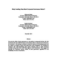
In Table 5 four-factor regression results are presented for the period 1990-1999 after forming hedge portfolios based on G index and E index levels. For the 1990-1999 period all difference portfolio alphas are positive and significant at the 1% level. The results 5 clearly show that during the 1990s good governance firms outperformed bad governance firms (whether G index or E index was used to proxy for firm governance) when controlling for factors previously shown to have power to predict future stock returns. With Table 5 alphas as our benchmarks we examine the 2000-2007 period and 1990-2007 period. In Table 6 four-factor regression results are presented for these periods after again forming hedge portfolios based on E index and G index levels. When E index is used to proxy for governance in the 2000-2007 period, the significance of the governance and stock return relationship is weakly present for extreme hedge portfolios but is mostly absent. Only 2 of 12 alphas are significant compared to 12 of 12 for the 1990-1999 period. The two significant alphas are for the value-weighted E index 0 – E index 5-6 and E index 0 – E index 4-5-6 hedge portfolios. These alphas are .45 and .43 respectively for the 2000-2007 period compared to 1.16 and .74 for the earlier period results presented in Table 5 and are significant at the 10% level rather than the 1% level. When G index is used to proxy for governance in the 2000-2007 period, alphas of both the equal- and value-weighted hedge portfolios are insignificant. Over the 1990-2007 period four-factor alphas are positive and significant at the 10% level or better for each of the 10 E index difference portfolios. 3 alphas are significant at the 1% level compared to 10 for the 1990-1999 period. The magnitudes of all alphas are reduced with reductions ranging from 31%-53% for value-weighted portfolios and 34%-49% for equal-weighted portfolios. Neither the equal- or valueweighted G index hedge portfolio alpha is significant. When governance is measured by E index levels the findings suggest good governance firms outperform bad governance firms over the full 1990-2007 period when controlling for the three factors of Fama and French and the Carhart momentum factor though this relationship is much less pronounced compared to the 1990-1999 period. There is again no evidence to suggest governance as measured by the G index is important for firm stock price performance over the 1990-2007 period. Calendar time regression analysis suggests governance is at least less important than suggested by prior literature. Though this relationship is still present when the E index is used to proxy for governance, it is nearly absent in the later period and is substantially weakened over the full sample period, suggesting full sample results may be driven by the 1990-1999 period. Given this, we next explore why results from the 1990-1999 period suggest such a strong relationship between firm governance and stock returns. Controlling for Portfolio Exchange Composition Figures 1-3 graph value-weighted buy-and-hold returns for extreme governance portfolios as well as hedge portfolios through time over the full 1990-2007 period. In Figures 1, 2 and 3 respectively buy-andhold returns are graphed for E index 0 and E index 5-6, E index 0 and E index 4-5-6, and G index 5 and G index 14 portfolios. In each case the good governance portfolio exhibits extremely high returns in the late 1990’s followed by negative returns through approximately the end of 2002. This return pattern is consistent with performance of the Nasdaq index over the same period which peaked in February 2000 and did not resume an upward trend until late 2002. Bad governance portfolios performed much more consistently over the late 1990s and early 2000s and portfolios values arguably followed a path more appealing to investors. In Figure 4 the percentage of E index 0 and E index 5-6 firms which are Nasdaq firms are presented for each data release year. With the exception of the 1993 announcement, the percentage of E index 0 firms which are Nasdaq firms is higher than the percentage for E index 5-6 firms. For the 1990, 1993, and 1995 announcements the percentages of firms which are Nasdaq firms are relatively even for the two portfolios. The percentage of E index 0 firms which are Nasdaq firms increases from 25% to 38% from the 1995 announcement to the 1998 announcement while the E Index 5-6 percentage remains nearly constant. In 1998 the percentage of E index 0 firms which are Nasdaq firms is 1.84 times the percentage for E index 5-6 firms. This increase occurs just before the period of high returns for the Nasdaq index when the superior performance of good governance firms relative to bad governance firms was most

Journal of Accounting and Finance Vol. 16(5) 2016

43

pronounced. Over all announcements the E index 0 portfolio has an average percentage of firms which are Nasdaq firms 1.71 times the percentage for the E index 5-6 portfolio. In Figure 5 the percentage of E index 0 and E index 4-5-6 firms which are Nasdaq firms are presented for each data release year. The relationship is slightly more pronounced than in Figure 4. For every announcement the percentage of E index 0 firms which are Nasdaq firms is higher than the percentage for E index 4-5-6 firms. In 1998 the percentage of E index 0 firms which are Nasdaq firms is 2.34 times the percentage for E index 4-5-6 firms. Over all announcements the E index 0 portfolio has an average percentage of firms which are Nasdaq firms 1.80 times the percentage for the E index 4-5-6 portfolio. In Figure 6 the percentage of G index 5 and G index 14 firms which are Nasdaq firms are presented for each data release year. The relationship of governance and portfolio exchange composition is strongest when governance is measured by G index. For every announcement the percentage of firms which are Nasdaq firms is higher for the G index 5 portfolio than for the G index 14 portfolio. In 1998 the percentage of G index 5 firms which are Nasdaq firms is 2.68 times the percentage for G index 14 firms. Over all announcements the G index 5 portfolio has an average percentage of firms which are Nasdaq firms 2.31 times the percentage for the G index 14 portfolio. It is clear from Figures 4-6 that good governance firms are much more likely than bad governance firms to be Nasdaq firms. Given the concentration on the 1990-1999 period in both BCF and GIM and evidence presented in Figures 1-3 it appears the findings in these studies are likely period specific and driven in part by differences in portfolio exchange composition. To further investigate this assertion mean returns over the 1990-1999 period are presented in Table 7 for extreme governance portfolios using all firms and after excluding Nasdaq firms. This analysis is performed using both equal- and value-weighting for the E Index 0 portfolio relative to the E index 5-6 portfolio, the E Index 0 portfolio relative to the E index 4-5-6 portfolio, and the G Index 5 portfolio relative to the G index 14 portfolio. When equal-weighting is used, excluding Nasdaq firms reduces the mean return difference slightly for the E index 0 portfolio relative to the E index 5-6 portfolio from .48% to .41% per month. When value-weighting is used the mean return difference is reduced from 1.01% to .76%. When comparing the E index 0 portfolio and the E index 4-5-6 portfolio, equal- and valueweighted mean return differences are reduced from .37% to .20% and from .72% to .46% respectively by excluding Nasdaq firms. Return differences are also reduced substantially for G index portfolios. When comparing the G index 5 portfolio and the G index 14 portfolio, equal- and value-weighted mean return differences are reduced from .35% to .00% and from .67% to .42% respectively. These results clearly show that Nasdaq firms played an important role is the observed relationships between firm governance and stock price performance in the 1990s. We should also point out the importance of weighting for portfolio return differences. When valueweighting the difference in mean monthly returns for the E index 0 portfolio relative to the E index 5-6 portfolio is 1.01%. When equal-weighting is used this difference is .48%. Similarly the mean monthly returns difference for the E index 0 portfolio relative to the E index 4-5-6 portfolio is reduced from .72% to .37% when equal-weighting rather than value-weighting is used. The same is true for the G index 5 and G index 14 portfolios, with a reduction from .67% to .35%. This suggests a few large firms may be important in driving the relationships between firm governance and stock price performance in the 1990s. Figures 7-9 graph equal-weighted buy-and-hold returns after excluding Nasdaq firms for extreme governance portfolios as well as hedge portfolios through time over the full 1990-2007 period. In Figures 7, 8 and 9 respectively E index 0 and E index 5-6, E index 0 and E index 4-5-6, and G index 5 and G index 14 portfolios buy-and-hold returns are graphed. In each figure, good and bad governance portfolio values move together closely. This is especially true in Figures 8 and 9 where returns for good and bad governance portfolio values move together almost identically. These figures are strong evidence that the relationship between firm governance and stock returns documented in BCF and GIM is period specific and driven by Nasdaq firms and large firms. We also perform calendar time regression analysis while controlling for portfolio exchange composition differences. This is accomplished in two ways. The first method is to exclude Nasdaq firms and employ the four-factor regression model specified in equation (1). The second method is the addition

44

Journal of Accounting and Finance Vol. 16(5) 2016

of a fifth factor to the three factors of Fama and French and momentum factor of Carhart in our regression model. The regression model with the added factor is given below. 𝐷𝐼𝐹𝐹𝑡 = 𝛼 + 𝛽1 𝑀𝐾𝑇𝑡 + 𝛽2 𝑆𝑀𝐵𝑡 + 𝛽3 𝐻𝑀𝐿𝑡 + 𝛽4 𝑈𝑀𝐷𝑡 + 𝛽5 𝑁𝐴𝑆𝑡 + 𝜀𝑡

(2)

NAS is the value-weighted monthly return of all Nasdaq firms listed on CRSP less the CRSP valueweighted monthly index return. The NAS factor is meant to control from the degree to which portfolio returns are related to returns on the Nasdaq index. The abnormal return for a portfolio is alpha from performing the regression in equation (1) or equation (2). Both regression models are used for equal- and value-weighted hedge portfolios including all firms as well as hedge portfolios excluding Nasdaq firms. In Table 8 portfolio alphas and coefficients of NAS are presented for hedge portfolios taking long positions in E index 0 firms and short positions in E index 5-6 firms. When all firms are included and regression model (2) is used alphas are insignificant and the coefficients of NAS are positive and significant for both equal- and value-weighted portfolios over the 1990-1999 and 1990-2007 periods. When Nasdaq firms are excluded and regression model (1) is used alphas are reduced slightly relative to those for portfolios including all firms but remain significant. In Table 9 portfolio alphas and coefficients of NAS are presented for the hedge portfolios taking long positions in E index 0 firms and short positions in E index 4-5-6 firms. Results are similar to those presented in Table 8. Again we see that when all firms are included and regression model (2) is used alphas are insignificant and the coefficients of NAS are positive and significant over both periods using both weighting methods. Reductions in alphas are more pronounced when Nasdaq firms are excluded than in Table 8. In Table 10 the analysis is repeated for G index difference portfolios. The coefficients of NAS are significant in each of the four cases when all firms are included. Either excluding Nasdaq firms or including the NAS factor results in insignificant alphas in all cases. While the significance of NAS coefficients is not surprising given differences in good and bad governance portfolio exchange composition, the resulting insignificant alphas for all difference portfolios, weighting methods and time periods provides more support for the importance of the Nasdaq bubble in the previously documented relationship between firm governance and stock returns. Overall, portfolio exchange composition analysis shows that Nasdaq firms played an important role in driving the results observed by GIM and BCF. Controlling for differences in portfolio exchange composition reduces or eliminates the significance of results presented in GIM and BCF in almost all cases. Given the differential performance of Nasdaq and non-Nasdaq firms over the late 1990s and early 2000s it is important to control for possible differences in portfolio exchange composition when analyzing portfolio returns over this period. CONCLUDING REMARKS Our findings suggest the previously documented superior performance of good governance firms relative to bad governance firms was a period specific result. Further, these results were partially driven by large firms and differences in portfolio exchange composition. We calculate extreme governance portfolio mean returns, hedge portfolio mean returns, and four-factor alphas over the 1990-2007 period and find the superior performance of good governance firms relative to bad governance firms is substantially reduced when E index score is used as a proxy for firm governance and is absent when G index score is used as a proxy for firm governance. Given the strong evidence of superior performance for good governance firms over the 1990-1999 period and subsequent reversal over the 2000-2007 period, we further examine the early period to determine why this superior performance was observed. We find two issues which largely contribute to this finding. Early period results were partially driven by large firms as evidenced by observation of a stronger relationship between firm governance and returns when value-weighted rather than equalweighted portfolio performance is examined. Also, the exchange compositions of good and bad governance portfolios vary greatly, with good governance firms being much more likely to be Nasdaq

Journal of Accounting and Finance Vol. 16(5) 2016

45

firms. When controlling for weighting and portfolio exchange composition issues, the significance of results documented in GIM and BCF are substantially reduced or eliminated. REFERENCES Bebchuk, L., & Cohen, A. (2005). The costs of entrenched boards, Journal of Financial Economics, 78, 409-433. Bebchuk, L., Cohen, A. & Ferrell, A. (2009). What matters in corporate governance?, Review of Financial Studies, 22, 783-827. Bhagat, S., & Bolton, B. (2008). Corporate Governance and Firm Performance. Journal of Corporate Finance, 14, 257–73. Byrd, J. W., & Hickman, K. (1992). Do outside directors monitor managers? Evidence from tender offer bids, Journal of Financial Economics, 32, 195-221. Carhart, M. (1997). On persistence in mutual fund performance, Journal of Finance, 52, 57–82. Coles, J. L., Lemmon, M.L. & Meschke, F. (2007). Structural models and endogeneity in corporate finance: The link between managerial ownership and corporate performance, Working paper, David Eccles School of Business, University of Utah. Core, J. E., Guay, W.R. & Rusticus, T.O. (2006). Does weak governance cause weak stock returns? An examination of firm operating performance and investors' expectations, The Journal of Finance, 61, 655-687. Cremers, M, & Nair, V.B. (2005). Governance mechanisms and equity prices, The Journal of Finance, 60, 2859-2894. Fama, E.F., & French, K.R. (1993). Common risk factors in the returns on bonds and stocks, Journal of Financial Economics, 33, 3–53. Gompers, P.A., Ishii, J.L. & Metrick, A. (2003). Corporate governance and equity prices, Quarterly Journal of Economics, 118, 107-155. Johnson, S.A., Moorman, T. & Sorescu, S.M. (2009). A reexamination of corporate governance and equity prices, Review of Financial Studies, 22, 4753-4786. Ofek, E, and Richardson, M. (2003). DotCom mania: The rise and fall of internet stock prices, Journal of Finance, 58, 1113–1137. Rosenstein, S. & Wyatt, J.G. (1990). Outside directors, board independence, and shareholder wealth, Journal of Financial Economics, 26, 175-192. Yermack, D. (1996). Higher market valuation for firms with a small board of directors, Journal of Financial Economics, 40, 185-211. Yermack, D. (2006). Flights of fancy: Corporate jets, CEO perquisites, and inferior shareholder returns, Journal of Financial Economics, 80, 211-242.

46

Journal of Accounting and Finance Vol. 16(5) 2016

APPENDIX TABLE 1 MEAN MONTHLY RETURNS BY E-INDEX 1990-1999

This table presents mean monthly returns for portfolios formed based on E Index levels over the period September 1990 – December 1999. Returns are presented using both equal- and valueweighting. For both equal- and value- weighted mean returns, the results of Bebchuk, Cohen, and Ferrell (2009) as well as a replication of their results are presented. We also include mean returns for the E index 4-5-6 portfolio. When calculating mean monthly value-weighted returns Bebchuk, Cohen, and Ferrell erred in using month t market equity rather than month t-1 market equity to weight month t returns. We also present corrected value-weighted mean returns using month t-1 market equity to weight month t returns. Firms are placed in E-index portfolios in September 1990, July 1993, July 1995 and February 1998 based on IRRC data releases and remain in portfolios until the next data release.

TABLE 2 MEAN MONTHLY RETURNS BY G-INDEX 1990-1999

This table presents mean monthly returns for portfolios formed based on G Index levels over the period September 1990 – December 1999. Returns are presented using both equal- and valueweighting. Firms with G index levels greater than or equal to 14 are assigned to the G index 14 portfolio. Firms with G index levels less than or equal to 5 are assigned to the G index 5 portfolio. Firms are placed in G index portfolios in September 1990, July 1993, July 1995 and February 1998 based on RiskMetrics data releases and remain in portfolios until the next data release.

Journal of Accounting and Finance Vol. 16(5) 2016

47

TABLE 3 MEAN MONTHLY RETURNS BY E-INDEX 2000-2007, 1999-2007

Entrenchment Index level

2000-2007 Equal-Weight Value-Weight

1990-2007 Equal-Weight Value-Weight

E-Index 5-6

1.18%

0.97%

1.25%

0.99%

E-Index 4-5-6

1.18%

0.68%

1.29%

1.00%

E-Index 4

1.18%

0.63%

1.30%

1.01%

E-Index 3

1.28%

0.58%

1.37%

1.02%

E-Index 2

1.16%

0.40%

1.36%

1.04%

E-Index 1

1.17%

0.15%

1.41%

0.93%

E-Index 0

1.12%

0.47%

1.40%

1.23%

E-Index 0 - E-Index 5-6

-0.06%

-0.49%

0.14%

0.24%

E-Index 0 - E-Index 4-5-6

-0.06%

-0.21%

0.11%

0.23%

This table presents mean monthly returns for portfolios formed based on E Index levels over the period January 2000 – December 2007 and the period September 1990 – December 2007. Returns are presented using both equaland value-weighting. For the January 2000 – December 2007 period firms are placed in E index portfolios in January 2000, February 2002, January 2004 and January 2006 based on IRRC data releases and remain in portfolios until the next data release. For the September 1990 – December 2007 period firms are placed in E index portfolios in September 1990, July 1993, July 1995, February 1998, November 1999, February 2002, January 2004 and January 2006 based on RiskMetrics data releases and remain in portfolios until the next data release.

TABLE 4 MEAN MONTHLY RETURNS BY G-INDEX 2000-2007, 1999-2007

Governance Index level

2000-2007 Equal-Weight Value-Weight

1990-2007 Equal-Weight Value-Weight

G-Index 14

1.19%

0.91%

1.28%

1.08%

G-Index 13

1.27%

0.51%

1.38%

1.08%

G-Index 12

1.03%

0.37%

1.26%

0.90%

G-Index 11

1.16%

0.43%

1.35%

1.11%

G-Index 10

1.19%

0.58%

1.26%

1.07%

G-Index 9

1.29%

0.39%

1.39%

0.99%

G-Index 8

1.26%

0.37%

1.44%

1.03%

G-Index 7

1.17%

0.31%

1.43%

1.12%

G-Index 6

1.13%

0.60%

1.40%

1.18%

G-Index 5

1.20%

0.30%

1.39%

1.06%

G-Index 5 - G-Index 14

0.00%

-0.61%

0.11%

0.02%

This table presents mean monthly returns for portfolios formed based on G Index levels over the period January 2000 – December 2007 and the period September 1990 – December 2007. Returns are presented using both equaland value-weighting. Firms with G index levels less than or equal to 5 are assigned to the G index 5 portfolio. Firms with G index levels greater than or equal to 14 are assigned to the G-index 14 portfolio. For the January 2000 – December 2007 period firms are placed in G index portfolios in January 2000, February 2002, January 2004 and January 2006 based on IRRC data releases and remain in portfolios until the next data release. For the September 1990 – December 2007 period firms are placed in G index portfolios in September 1990, July 1993, July 1995, February 1998, November 1999, February 2002, January 2004 and January 2006 based on RiskMetrics data releases and remain in portfolios until the next data release.

48

Journal of Accounting and Finance Vol. 16(5) 2016

Journal of Accounting and Finance Vol. 16(5) 2016

49

(0.22)

0.45

(0.079)

0.25

(0.106)

0.32

(0.138)

0.41

(0.134)

**

***

***

***

***

***

(0.22)

0.48

(0.087)

0.24

(0.112)

0.31

(0.146)

0.41

(0.152)

0.42

(0.217)

0.61

**

***

***

***

***

***

Replication

(0.26)

0.71

(0.116)

0.47

(0.141)

0.52

(0.153)

0.62

(0.191)

0.74

(0.284)

1.16

BCF/GIM

***

***

***

***

***

***

(0.25)

0.69

(0.135)

0.46

(0.157)

0.51

(0.172)

0.62

(0.203)

0.74

(0.290)

1.16

***

***

***

***

***

***

Replication

Value-Weight

(0.127)

0.46

(0.151)

0.52

(0.162)

0.63

(0.197)

0.84

(0.282)

1.24

Corrected

***

***

***

***

***

This table presents four-factor regression alphas for the period 1990-1999 after placing firms in portfolios based on E index and G index levels. Abnormal returns for each portfolio are formed by taking long positions in firms with low E index (G index) levels and short firms with high E index (G index) levels. Abnormal returns are then calculated as alphas from the following regression model 𝐷𝐼𝐹𝐹𝑡 = 𝛼 + 𝛽1 𝑀𝐾𝑇𝑡 + 𝛽2 𝑆𝑀𝐵𝑡 + 𝛽3 𝐻𝑀𝐿𝑡 + 𝛽4 𝑈𝑀𝐷𝑡 + 𝜀𝑡 . For each E index (G index) level portfolio we calculate equal- and value-weighted mean monthly returns and then take the difference of various portfolio returns as our dependent variable, DIFF. MKT is the monthly CRSP value-weighted index return less the risk-free rate. SMB and HML are the monthly size and book-to-market equity return factors presented in Fama and French (1993). UMD is the momentum factor presented in Carhart (2007). * is significant at the 10% level, ** is significant at the 5% level, *** is significant at the 1% level.

G-Index 5 - G-Index 14

E Index 0-1-2 - E Index 3-4-5-6

E Index 0-1 - E Index 3-4-5-6

E Index 0-1 - E Index 4-5-6

0.42

(0.200)

0.61

E Index 0 - E Index 5-6

E Index 0 - E Index 4-5-6

BCF/GIM

Long-short portfolios

Equal-Weight

TABLE 5 FOUR FACTOR HIGH-LOW PORTFOLIO ALPHAS BY E INDEX AND G INDEX 1990-1999

TABLE 6 FOUR FACTOR HIGH-LOW PORTFOLIO ALPHAS BY E INDEX AND G INDEX Equal-Weight Long-short portfolios E Index 0 - E Index 5-6 E Index 0 - E Index 4-5-6 E Index 0-1 - E Index 4-5-6 E Index 0-1 - E Index 3-4-5-6 E Index 0-1-2 - E Index 3-4-5-6 G-Index 5 - G-Index 14

2000-2007

Value-Weight

1990-2007

0.302

0.345

(0.243)

(0.159)

0.218

0.229

(0.200)

(0.125)

0.259

0.268

(0.163)

(0.110)

0.124

0.180

(0.144)

(0.090)

**

2000-2007 0.449

*

**

**

*

0.425

0.778

*

0.576

(0.237)

(0.147)

0.093

0.313

(0.167)

(0.114)

0.079

0.253

(0.166)

(0.112)

0.046

0.215 (0.094)

0.071

0.121

(0.118)

(0.072)

(0.134)

0.094

0.229

(0.232)

0.177

(0.227)

(0.154)

(0.287)

(0.187)

This table presents four-factor regression alphas for the periods 1990-2007, and 2000-2007 after placing firms in portfolios based on E index and G index levels. Abnormal returns for each portfolio are formed by taking long positions in firms with low E index (G index) levels and short firms with high E index (G index) levels. Abnormal returns are then calculated as alphas from the following regression model 𝐷𝐼𝐹𝐹𝑡 = 𝛼 + 𝛽1 𝑀𝐾𝑇𝑡 + 𝛽2 𝑆𝑀𝐵𝑡 + 𝛽3 𝐻𝑀𝐿𝑡 + 𝛽4 𝑈𝑀𝐷𝑡 + 𝜀𝑡 . For each E index (G index) level portfolio we calculate equal- and value-weighted mean monthly returns and then take the difference of various portfolio returns as our dependent variable, DIFF. MKT is the monthly CRSP value-weighted index return less the risk-free rate. SMB and HML are the monthly size and bookto-market equity return factors presented in Fama and French (1993). UMD is the momentum factor presented in Carhart (2007). * is significant at the 10% level, ** is significant at the 5% level, *** is significant at the 1% level.

50

Journal of Accounting and Finance Vol. 16(5) 2016

***

(0.198)

(0.257) *

1990-2007

***

***

**

**

TABLE 7 MEAN MONTHLY HIGH-LOW RETURNS BY EXCHANGE 1990-1999

All Firms

Equal Weight Excluding Nasdaq

All - Excl. Nasdaq

All Firms

Value-Weight Excluding Nasdaq

All - Excl. Nasdaq

E-Index 0

1.74%

1.48%

0.26%

1.98%

1.70%

0.28%

E-Index 5-6

1.26%

1.07%

E-Index 0 - E-Index 5-6

0.48%

0.41%

0.19%

0.97%

0.94%

0.03%

1.01%

0.76%

All Firms

Excluding Nasdaq

All - Excl. Nasdaq

All Firms

Excluding Nasdaq

All - Excl. Nasdaq

E-Index 0

1.74%

1.48%

0.26%

1.98%

1.70%

0.28%

E-Index 4-5-6 E-Index 0 - E-Index 4-5-6

1.37%

1.27%

0.10%

1.27%

1.24%

0.03%

0.37%

0.20%

0.72%

0.46%

All Firms

Excluding Nasdaq

All - Excl. Nasdaq

All Firms

Excluding Nasdaq

All - Excl. Nasdaq

G-Index 5

1.67%

1.27%

0.40%

1.85%

1.59%

0.26%

G-Index 14

1.32%

1.27%

0.05%

1.18%

1.17%

0.01%

G-Index 5 - G-Index 14

0.35%

0.00%

0.67%

0.42%

This table presents mean monthly returns for portfolios formed based on G Index and E index levels over the period September 1990 – December 1999. Returns are presented using both equal- and value-weighting and including and excluding Nasdaq firms. Firms with G index (E index) levels greater than or equal to 14 (equal to 4, 5, and 6) are assigned to the G index 14 (E index 4-5-6) portfolio. Firms with G index (E index) levels less than or equal to 5 (equal to 0) are assigned to the G index 5 (E index 0) portfolio. Firms are placed in G index (E index) portfolios in September 1990, July 1993, July 1995 and February 1998, November 1999 based on RiskMetrics data releases and remain in portfolios until the next data release.

Journal of Accounting and Finance Vol. 16(5) 2016

51

TABLE 8 FOUR FACTOR HIGH-LOW PORTFOLIO ALPHAS FOR E INDEX 0 – E INDEX 5-6 Equal-Weight Alpha 1990s All Firms 1990s Excluding NASDAQ Full Sample All Firms Full Sample Excluding NASDAQ

0.606

NAS

***

0.375 ***

0.491

**

0.345

**

0.088

*

0.092 0.396

***

**

0.224

Alpha 1.242

0.226

0.585

0.343

Value-Weight

0.184

**

NAS

***

0.373 0.936

***

0.536

*

0.778

***

0.292 0.605

***

0.405

**

0.850

***

0.391

***

0.748

***

0.308

***

This table presents four-factor regression alphas for the periods 1990-2007, and 2000-2007. Abnormal returns for each portfolio are formed by taking long positions in firms with low E index levels (E Index 0) and short firms with high E index levels (E Index 5-6). Abnormal returns are then calculated as alphas from the following regression model 𝐷𝐼𝐹𝐹𝑡 = 𝛼 + 𝛽1 𝑀𝐾𝑇𝑡 + 𝛽2 𝑆𝑀𝐵𝑡 + 𝛽3 𝐻𝑀𝐿𝑡 + 𝛽4 𝑈𝑀𝐷𝑡 + 𝛽5 𝑁𝐴𝑆𝑡 + 𝜀𝑡 . For each E index level portfolio we calculate equal- and value-weighted mean monthly returns and then take the difference of various portfolio returns as our dependent variable, DIFF. MKT is the monthly CRSP value-weighted index return less the risk-free rate. SMB and HML are the monthly size and book-to-market equity return factors presented in Fama and French (1993). UMD is the momentum factor presented in Carhart (2007). NAS is the value-weighted monthly return of all Nasdaq firms listed on CRSP less the CRSP value-weighted monthly index return. Abnormal return alphas are presented including and excluding the NAS factor and including and excluding Nasdaq firms. * is significant at the 10% level, ** is significant at the 5% level, *** is significant at the 1% level.

52

Journal of Accounting and Finance Vol. 16(5) 2016

TABLE 9 FOUR FACTOR HIGH-LOW PORTFOLIO ALPHAS FOR E INDEX 0 – E INDEX 4-5-6 Equal-Weight Alpha 1990s All Firms 1990s Excluding NASDAQ Full Sample All Firms Full Sample Excluding NASDAQ

0.415

0.313 0.132

0.164 0.043

*

*

-0.036

Alpha 0.839

***

**

0.152 0.229

NAS

***

0.095 0.287

Value-Weight

0.408

***

*

0.186

***

NAS

***

0.104 0.536

***

0.280

*

0.576

***

0.189 0.389

***

0.269

**

0.719

***

0.251

***

0.596

***

0.186

***

This table presents four-factor regression alphas for the periods 1990-2007, and 2000-2007. Abnormal returns for each portfolio are formed by taking long positions in firms with low E index levels (E Index 0) and short firms with high E index levels (E Index 4-5-6). Abnormal returns are then calculated as alphas from the following regression model 𝐷𝐼𝐹𝐹𝑡 = 𝛼 + 𝛽1 𝑀𝐾𝑇𝑡 + 𝛽2 𝑆𝑀𝐵𝑡 + 𝛽3 𝐻𝑀𝐿𝑡 + 𝛽4 𝑈𝑀𝐷𝑡 + 𝛽5 𝑁𝐴𝑆𝑡 + 𝜀𝑡 . For each E index level portfolio we calculate equal- and value-weighted mean monthly returns and then take the difference of various portfolio returns as our dependent variable, DIFF. MKT is the monthly CRSP value-weighted index return less the risk-free rate. SMB and HML are the monthly size and book-to-market equity return factors presented in Fama and French (1993). UMD is the momentum factor presented in Carhart (2007). NAS is the value-weighted monthly return of all Nasdaq firms listed on CRSP less the CRSP value-weighted monthly index return. Abnormal return alphas are presented including and excluding the NAS factor and including and excluding Nasdaq firms. * is significant at the 10% level, ** is significant at the 5% level, *** is significant at the 1% level.

Journal of Accounting and Finance Vol. 16(5) 2016

53

TABLE 10 FOUR FACTOR HIGH-LOW PORTFOLIO ALPHAS FOR G INDEX 5 – G INDEX 14 Equal-Weight Alpha 1990s All Firms 1990s Excluding NASDAQ Full Sample All Firms Full Sample Excluding NASDAQ

0.478

Value-Weight

NAS

**

0.172

0.692 0.299

**

0.194 0.145

0.047

0.407

0.360

***

*

0.035

0.177 0.383

***

0.159

**

0.028 -0.075

NAS

***

0.324 0.442

0.229 -0.020

Alpha

-0.126

0.466

***

0.085 0.096

-0.017

This table presents four-factor regression alphas for the periods 1990-2007, and 2000-2007. Abnormal returns for each portfolio are formed by taking long positions in firms with low G index levels (G Index less than or equal to 5) and short firms with high G index levels (G Index greater than or equal to 14). Abnormal returns are then calculated as alphas from the following regression model 𝐷𝐼𝐹𝐹𝑡 = 𝛼 + 𝛽1 𝑀𝐾𝑇𝑡 + 𝛽2 𝑆𝑀𝐵𝑡 + 𝛽3 𝐻𝑀𝐿𝑡 + 𝛽4 𝑈𝑀𝐷𝑡 + 𝛽5 𝑁𝐴𝑆𝑡 + 𝜀𝑡 . For each G index level portfolio we calculate equal- and value-weighted mean monthly returns and then take the difference of various portfolio returns as our dependent variable, DIFF. MKT is the monthly CRSP value-weighted index return less the risk-free rate. SMB and HML are the monthly size and book-to-market equity return factors presented in Fama and French (1993). UMD is the momentum factor presented in Carhart (2007). NAS is the value-weighted monthly return of all Nasdaq firms listed on CRSP less the CRSP value-weighted monthly index return. Abnormal return alphas are presented including and excluding the NAS factor and including and excluding Nasdaq firms. * is significant at the 10% level, ** is significant at the 5% level, *** is significant at the 1% level.

54

Journal of Accounting and Finance Vol. 16(5) 2016

FIGURE 1 BUY AND HOLD VALUE-WEIGHTED PORTFOLIO RETURNS, E INDEX, ALL FIRMS

This figure graphs value-weighted buy-and-hold returns for portfolios formed based on E Index levels over the period September 1990 – December 2007. Extreme governance E Index high minus low hedge portfolios are formed by taking long positions in firms with low E index levels (E Index 0) and short positions in firms with high E index levels (E Index 5-6).

FIGURE 2 BUY AND HOLD VALUE-WEIGHTED PORTFOLIO RETURNS, E INDEX, ALL FIRMS

This figure graphs value-weighted buy-and-hold returns for portfolios formed based on E Index levels over the period September 1990 – December 2007. Extreme governance E Index high minus low hedge portfolios are formed by taking long positions in firms with low E index levels (E Index 0) and short positions in firms with high E index levels (E Index 4-5-6).

Journal of Accounting and Finance Vol. 16(5) 2016

55

FIGURE 3 BUY AND HOLD VALUE-WEIGHTED PORTFOLIO RETURNS, G INDEX, ALL FIRMS

This figure graphs value-weighted buy-and-hold returns for portfolios formed based on G Index levels over the period September 1990 – December 2007. For the September 1990 – December 2007 period firms are placed in G index portfolios in September 1990, July 1993, July 1995, February 1998, November 1999, February 2002, January 2004 and January 2006 based on RiskMetrics data releases and remain in portfolios until the next data release. Extreme governance G Index high minus low hedge portfolios are formed by taking long positions in firms with low G index levels (G Index less than or equal to 5) and short positions in firms with high G index levels (G Index greater than or equal to 14).

FIGURE 4 PERCENTAGE OF E INDEX FIRMS WHICH ARE NASDAQ FIRMS

This figure presents the percentage of sample firms in the extreme governance E Index portfolios which are Nasdaq firms over the period September 1990 – December 2007. For the September 1990 – December 2007 period, firms are placed in low E Index (E Index 0) and high E Index (E Index 5-6) portfolios in September 1990, July 1993, July 1995, February 1998, November 1999, February 2002, January 2004 and January 2006 based on RiskMetrics data releases and remain in portfolios until the next data release.

56

Journal of Accounting and Finance Vol. 16(5) 2016

FIGURE 5 PERCENTAGE OF E INDEX FIRMS WHICH ARE NASDAQ FIRMS

This figure presents the percentage of sample firms in the extreme governance E Index portfolios which are Nasdaq firms over the period September 1990 – December 2007. For the September 1990 – December 2007 period, firms are placed in low E Index (E Index 0) and high E Index (E Index 4-5-6) portfolios in September 1990, July 1993, July 1995, February 1998, November 1999, February 2002, January 2004 and January 2006 based on RiskMetrics data releases and remain in portfolios until the next data release.

FIGURE 6 PERCENTAGE OF G INDEX FIRMS WHICH ARE NASDAQ FIRMS

This figure presents the percentage of sample firms in the extreme governance G Index portfolios which are Nasdaq firms over the period September 1990 – December 2007. For the September 1990 – December 2007 period, firms are placed in low G Index (G Index less than or equal to 5) and high G Index (G Index greater than or equal to 14) portfolios in September 1990, July 1993, July 1995, February 1998, November 1999, February 2002, January 2004 and January 2006 based on RiskMetrics data releases and remain in portfolios until the next data release.

Journal of Accounting and Finance Vol. 16(5) 2016

57

FIGURE 7 BUY AND HOLD EQUAL-WEIGHTED PORTFOLIO RETURNS, E INDEX, EXCLUDING NASDAQ FIRMS

This figure graphs equal-weighted buy-and-hold returns after excluding Nasdaq firms, for portfolios formed based on E Index levels over the period September 1990 – December 2007. Extreme governance E Index high minus low hedge portfolios are formed by taking long positions in firms with low E index levels (E Index 0) and short positions in firms with high E index levels (E Index 5-6).

FIGURE 8 BUY AND HOLD EQUAL-WEIGHTED PORTFOLIO RETURNS, E INDEX, EXCLUDING NASDAQ FIRMS

This figure graphs equal-weighted buy-and-hold returns after excluding Nasdaq firms, for portfolios formed based on E Index levels over the period September 1990 – December 2007. Extreme governance E Index high minus low hedge portfolios are formed by taking long positions in firms with low E index levels (E Index 0) and short positions in firms with high E index levels (E Index 4-5-6).

58

Journal of Accounting and Finance Vol. 16(5) 2016

FIGURE 9 BUY AND HOLD EQUAL-WEIGHTED PORTFOLIO RETURNS, G INDEX, EXCLUDING NASDAQ FIRMS

This figure graphs equal-weighted buy-and-hold returns after excluding Nasdaq firms, for portfolios formed based on G Index levels over the period September 1990 – December 2007. For the September 1990 – December 2007 period firms are placed in G index portfolios in September 1990, July 1993, July 1995, February 1998, November 1999, February 2002, January 2004 and January 2006 based on RiskMetrics data releases and remain in portfolios until the next data release. Extreme governance G Index high minus low hedge portfolios are formed by taking long positions in firms with low G index levels (G Index less than or equal to 5) and short positions in firms with high G index levels (G Index greater than or equal to 14).

Journal of Accounting and Finance Vol. 16(5) 2016

59