DO POLITICAL PARTIES MATTER? EVIDENCE FROM U.S. CITIES∗ FERNANDO FERREIRA AND JOSEPH GYOURKO Are cities as politically polarized as states and countries? “No” is the answer from our regression discontinuity design analysis, which shows that whether the mayor is a Democrat or a Republican does not affect the size of city government, the allocation of local public spending, or crime rates. However, there is a substantial incumbent effect for mayors. We investigate three mechanisms that could account for the striking lack of partisan impact at the local level, and find the most support for Tiebout competition among localities within metropolitan areas.
I. INTRODUCTION Recent research in political economy concludes that political partisanship influences politicians’ voting behavior and policy outcomes at the national and state levels of government. Besley and Case (2003) use standard multivariate regression techniques, controlling for state and year fixed effects, to show that a higher fraction of Democrat party seats in the state legislature is associated with significantly higher state spending per capita, with about one-third of the increase attributable to greater expenditures on family assistance. Lee, Moretti, and Butler (2004) exploit the random variation associated with close U.S. congressional elections in a regression discontinuity (RD) research design to show that party affiliation explains a very large fraction of the variation in Congressional voting behavior, and that voters essentially are electing policies proposed by political parties instead of affecting the policy positions of the parties.1 ∗ The authors thank the Research Sponsor Program of the Zell/Lurie Real Estate Center at Wharton for financial support. Misha Dworsky, Andrew Moore, Bob Jobim, and Igar Fuki provided outstanding research assistance. We also appreciate the comments and suggestions of the editor (Ed Glaeser) and referees, as well as Claudio Ferraz, Bob Inman, David Lee, and seminar participants at the Wharton Applied Economics Workshop, Carnegie Mellon, Columbia University, Duke University, the Federal Reserve Bank of Philadelphia, IPEA–Rio de Janeiro, the University of California–Berkeley, the University of Southern California, and the University of Toronto. 1. There is now a consensus that U.S. congressional voting behavior is highly partisan, with Lee, Moretti, and Butler’s new research design confirming previous results (e.g., Poole and Rosenthal [1984]; Snyder and Groseclose [2000]). The evidence regarding the policy impact of which party occupies the presidency is more mixed, partly due to the difficulty of establishing robust relationships given the small number of Presidential elections (Alesina, Roubini, and Cohen 1997). Recently, Snowberg, Wolfers, and Zitzewitz (2007) used high-frequency data from prediction markets to get around this problem and found that expectations about which party would control the executive branch of government in the 2004 C 2009 by the President and Fellows of Harvard College and the Massachusetts Institute of �
Technology. The Quarterly Journal of Economics, February 2009
399
400
QUARTERLY JOURNAL OF ECONOMICS
We use a new data set for mayoral elections to study the impact of political partisanship at the local level in the United States. To deal with the endogeneity of party affiliation of the mayor in a city, we employ the RD approach on nearly 2,000 direct mayoral elections in over 400 U.S. cities between 1950 and 2000. Comparing cities where Democrats barely won an election with cities where Democrats barely lost, we find virtually no partisan differences in policy outcomes at the municipal level. Whether the mayor is a Democrat or Republican has little or no impact on the size of local government, the composition of local public expenditures, or the crime rate.2 These RD results are stable across a variety of robustness checks, and they are markedly different from na¨ıve ordinary least squares (OLS) estimators, which yield significant differences between the two major parties in the size of local government. Although there is no partisan impact on the policy outcomes we observe at the local level, there is a substantial advantage to incumbency that is similar in magnitude to that reported for U.S. congressional representatives (Lee 2001, 2008). Democratic mayors enjoy about a one-third higher probability of winning the next election if they personally or someone from their party already occupies the office. We also investigate three potential explanations for the striking lack of partisanship at the local level. The first is that cities simply are more homogeneous than higher levels of government. Both citizen candidate (Alesina 1988; Besley and Coate 1997) and targeted strategic extremism (Glaeser, Ponzetto, and Shapiro 2005) models would predict less partisanship in such an environment. A second possible explanation arises from the fact that cities face constraints that are different from those relevant to higher levels of government. If exit is more readily achievable by voters at the local level because there are plentiful nearby jurisdictions
presidential election influenced various market prices and indexes. At the state level, Besley and Case’s (2003) review of the literature notes several other studies that find a material impact of political partisanship on fiscal outcomes (e.g., Grogan [1994], Besley and Case [1995], and Knight [2000]). 2. Research on the impact of local politics in foreign countries is more prevalent because of superior local elections data outside the United States. Bertrand and Kramarz (2002) analyze the influence of parties on local zoning boards in France, finding that more restrictive zoning leads to less long-term growth. Pettersson-Lidbom (2008) finds that party labels matter at the local level in Sweden, with cities in which the majority of council representatives belong to left-wing parties having both higher spending and taxes than cities where the majority belong to right-wing parties. Hence, our finding of no partisan impact differs from those reported in non-U.S. studies.
DO POLITICAL PARTIES MATTER?
401
within the labor market area, municipal competition may lead to less partisanship (Peterson 1981). Other constraints could involve institutional rules, such as more binding balanced budget provisions that reduce the scope for partisan behavior. A third possible explanation is that it is not feasible to send the type of targeted messages to specific voters within a city that Glaeser, Ponzetto, and Shapiro (2005) argue are necessary for partisanship to have a high payoff. We test the relevance of these three theories empirically within our RD design. The evidence is most consistent with Tiebout competition being the primary mechanism by which partisanship is disciplined at the local level. Having elected a Democrat in a closely contested mayoral race is associated with a 7%–9% larger government only for cities with few competing jurisdictions nearby relative to otherwise similar cities located in more jurisdictionally fragmented metropolitan areas. We find no evidence that city-level income homogeneity or an inability to target messages precisely impacts partisanship at the local level, but this remains an issue in need of more research. Overall, our estimates not only show that local partisanship effects are very different from what has been documented at other levels of government, but also that the mechanisms leading to convergence in policy outcomes can be specific to the local environment. Hence, caution should be used when generalizing political economy theories that may be specific to a certain branch or level of government. The plan of the paper is as follows. The next section discusses why political partisanship could have different impacts in cities versus states or countries. This is followed in Section III with a description of the new data used in our empirical analysis. The main results on partisan differences in terms of the size of local government, crime rates, and the composition of its spending are reported and discussed in Section IV. An analysis of the mechanisms leading to reduced partisanship at the local level is reported in Section V. There is a brief conclusion. II. WHY MIGHT PARTISAN POLITICAL IMPACTS BE DIFFERENT AT THE LOCAL LEVEL? For many years, the theoretical consensus among political economists was that the impact of partisanship on policy outcomes was limited or nil (Hotelling 1929; Downs 1957). This stood in stark contrast to the growing body of empirical evidence discussed
402
QUARTERLY JOURNAL OF ECONOMICS
above that partisan impacts are strong at the state and federal levels of government. Two types of models were proposed to account for this. One reflects a taste-based mechanism that can arise from candidate or party policy preferences (Alesina 1988; Besley and Coate 1997).3 In this framework, if candidates or parties care about certain outcomes and they cannot credibly commit to moderate policies, there will be divergence in policy space. Glaeser, Ponzetto, and Shapiro (2005) provide a different rationale, showing that staking out extreme policy positions can be beneficial to a party if it can strategically target messages to its supporters so that donations or turnout increase sufficiently to affect the probability of winning elections. An important initial question is whether there is any reason to suspect that partisan political impacts at the local level would be different from those found at higher levels of government. The answer is “yes” because of the very different economic and political environments in which cities exist and operate. Most localities are part of a larger labor market (or metropolitan) area. Moving costs are relatively low within metropolitan areas, which can facilitate spatial sorting into specific types of communities, as envisaged by Charles Tiebout (1956). This suggests that the populations of cities are likely to be more homogeneous than those of congressional districts or states. We document below that this is indeed the case. Both types of models discussed above are likely to predict less partisanship the more alike are the residents of any jurisdiction. For example, greater homogeneity among citizens may facilitate political parties credibly committing to moderate policies according to “citizen-candidate” models. City homogeneity also can limit strategic extremism, because it becomes harder to win elections by catering to a thin minority with extreme preferences in such circumstances. A Tiebout-type urban setting also suggests a different competitive environment among cities within the same metropolitan area than among states within the same country. More intense competition among jurisdictions may restrict a politician’s desire or ability to pursue highly partisan policies if residents can readily move to a nearby town. Whether “Tiebout even needs politics” has long been debated in urban economics (Epple and Zelenitz 1981; Henderson 1985). This issue has been studied by political 3. Also, see Wittman (1977, 1983) for early work on politicians’ tastes and partisanship.
DO POLITICAL PARTIES MATTER?
403
scientists, too, with Peterson (1981) arguing that the competitive nature of the American urban environment limits the scope for redistribution at the local level. If this leads to a heightened emphasis on competence in the provision of basic services, the political gains to partisan behavior could be smaller at the local level of government. The constraints need not be exclusively related to Tiebout competition, either. For example, balanced budget rules or scarce intergovernmental aid to cities also could limit the scope for redistribution. It is also possible that the smaller physical sizes and populations of cities and towns limit the strategic effectiveness of partisanship, independent of population homogeneity. One needs to be able to precisely target messages to specific voters or there will not be any significant payoff from strategic extremism of the type proposed by Glaeser, Ponzetto, and Shapiro (2005). Limited variety in media at the metropolitan-area level could be a factor in this respect. If there is only one major daily newspaper serving all the towns in a metropolitan area, one cannot use it to send targeted messages to select voters. The types of policies relevant to local government also could play a role in mitigating the effectiveness of strategic extremism at the city level. Glaeser and Ward (2006) maintain that it is social issues that essentially define partisan differences in American political life. However, these are not really under local control. Economic responsibilities such as the provision of basic services and local taxes, not abortion or the right to bear arms, are the province of city government. If the political divide is not wide on the issues central to local government, partisanship is less useful as an electoral strategy. In sum, it should not be presumed that the strong partisan impacts on policy outcomes reported at the state and federal levels of government also exist in cities. Independent analysis must be performed, and for that, new data are required. It is to that issue that we now turn.
III. DATA DESCRIPTION III.A. Mayoral Elections Survey Data The mayoral election data used in this paper were collected from a survey sent to all cities and townships in the United States with more than 25,000 people as of the year 2000. We requested comprehensive information on the timing (year and month) of all
404
QUARTERLY JOURNAL OF ECONOMICS
mayoral elections since 1950, the name of the mayor and secondplace candidate, aggregate vote totals and vote totals for each candidate, party affiliation, type of election, and some additional information pertaining to specific events such as runoffs and special elections.4 The final sample used in this paper consists of elections held in 413 cities between 1950 and 2005.5 The first column of Table I reports summary statistics on these cities as of the year 2000. Because we are keenly interested in the representativeness of our sample, the remaining columns report analogous information on different samples of cities. The second column reports data on the universe of 34,574 American cities. Given our 25,000 population cut-off, it is not surprising that the cities in our sample are more populous than the typical jurisdiction in the country. Bigger cities also tend to have better educated households that earn more money and live in more expensive houses. They also have more minority households, as indicated by the much larger share of the African-American population. Regionally, our sample is more heavily weighted toward the West and South, with there apparently being several small towns in the Midwest and North regions that we did not survey. More relevant is how representative our sample is compared to all 1,893 municipalities with more than 25,000 residents in the year 2000 (column (3)). Our sample has larger populations on average, but these two groups are similar in many ways. Not all cities directly elect a mayor, and column (4) reports information on the 877 cities that do so.6 Our final sample is very similar to this group of cities in demographic, economic, and geographic terms. From survey responses, we were able to obtain at least 4. The strengths of this survey compared to other publicly available data are numerous. The Municipal Yearbook only records the name of the current mayor for a given year, without specifying the year of election. The International City Managers Association (ICMA) only collects data on type of election and organizational features of cities every five years, without asking any question related to election outcomes. The Census of Governments also collects some information about type of election, as well as data on the race and sex of elected officials. Generally, political affiliation is not recorded in these sources. 5. All results reported in this paper are based on data collected through August 2007. Data collection efforts are ongoing, so the sample will be updated periodically. The data are available upon request. 6. In some cities, the mayor is appointed by or from the city council, whereas others hire a professional manager to run the locality. The total number of cities that elect a mayor is an estimate that was backed out from three different sources: Census of Governments, ICMA, and our own survey. Given that we find some discrepancies among these three sources, it is likely that the total number of such cities is slightly larger than 877.
DO POLITICAL PARTIES MATTER?
405
TABLE I SAMPLE REPRESENTATIVENESS
Final sample (1) Number of cities 413 Population 126,364 (256,768) % west 0.20 (0.40) % south 0.26 (0.44) % north 0.16 (0.36) % white 0.68 (0.22) % black 0.13 (0.17) % college degree 0.26 (0.13) Median family $53,035 income (16,202) Median house $132,622 value (66,582)
Cities Cities with Cities >25,000, All U.S. with >25,000 >25,000, elected mayor, cities population elected mayor survey reply (2) (3) (4) (5) 34,574 7,666 (62,732) 0.12 (0.33) 0.24 (0.43) 0.23 (0.42) 0.88 (0.20) 0.05 (0.14) 0.17 (0.13) $46,916 (19,262) $100,526 (86,412)
1,893 86,245 (255,000) 0.24 (0.42) 0.24 (0.43) 0.25 (0.43) 0.75 (0.19) 0.11 (0.16) 0.28 (0.15) $57,927 (19,566) $156,718 (100,769)
877 112,392 (346,409) 0.18 (0.39) 0.25 (0.44) 0.23 (0.42) 0.69 (0.23) 0.13 (0.17) 0.26 (0.13) $53,334 (16,687) $133,838 (70,988)
498 113,104 (234,874) 0.21 (0.41) 0.29 (0.45) 0.14 (0.35) 0.68 (0.22) 0.12 (0.17) 0.26 (0.13) $53,428 (16,265) $134,067 (66,961)
Notes. All variables are based on the 2000 Census. Standard deviations in parentheses. Column (1) presents descriptives for the mayoral election sample used in this paper. Column (2) reports descriptives for all cities in the United States. Column (3) restricts the sample to cities with more than 25,000 people as of year 2000. Column (4) additionally constrains the sample to cities that directly elect a mayor. Column (5) presents results for cities that replied to the survey with vote totals but no information about party affiliation. See the text for additional details.
some information on vote totals and candidate names for 57% of the 877 cities that elect mayors by popular vote. Summary statistics for this group of 498 places are displayed in column (5). Our final sample of 413 cities, which is 47% of those places that directly elect a mayor, also contains information on party affiliation, not just vote totals.7 7. Two factors made it difficult to collect information on candidates’ party affiliations, even when we knew who they were and how many people voted for them. First, some cities and counties could not provide the data because this required gathering information from inaccessible voter registration records. Second, there is a large fraction of cities (59% as of year 2000) that are institutionally nonpartisan in that they prohibit party labels from being printed on election ballots or used in election campaigning. This certainly does not mean that nearly 60% of mayoral races literally had no partisan content. A quick review showed that elections in many such cities (e.g., Los Angeles, California) clearly were partisan in the standard use of that term. Hence, survey information was complemented
406
QUARTERLY JOURNAL OF ECONOMICS
Our sample grows over time, and there is a cyclical pattern due to a large fraction of cities having two-year term elections. Fifty-one percent of our elections are for four-year terms, but 44% are for two years only, with 4% being for three-year terms. Although this means that we work with an unbalanced panel, this feature of the data is not a concern for our research design. With respect to party affiliation, 51% of the winners in our sample were Democrats, with 40% being Republicans. Over time, the proportion of Republican mayors has increased substantially. This change is due primarily to an increasing number of wins by Republican candidates, but also reflects an increase in the proportion of independent mayors or mayors from other parties. The sample of elections used in the regression discontinuity design estimates is restricted to 1,886 elections because we also eliminate races where mayors or second-place candidates were from third parties, when both mayor and runner-up candidate belong to the same party, or when a candidate runs unopposed. In addition, we only use elections that we were able to match with the fiscal data described below. III.B. Local Public Finance Data Information on a variety of local public finance variables is merged with the election data. The public finance data span the fiscal years 1950–2005 and are from the Historical Data Base of Individual Government Finances.8 These data are based on a Census of Governments conducted every five years, from the Annual Survey of Governments collected in every noncensus year, and are complemented by state data provided by the Census Bureau. The local public finance variables include measures of total revenues and taxes, the share of revenues due to intergovernmental transfers, spending (on current operations and capital goods, not including retirement and insurance expenses), employment (fulland part-time), as well as distributional data regarding shares of spending on labor, public safety, and parks and recreation.
by online searches for the party affiliation of candidates in “nonpartisan” cities by accessing restricted content of local newspapers from News Bank. Approximately 30% of the party affiliation data for nonpartisan cities were found with one of the methods above. The remaining 70% were collected directly from city or county clerks who were able to access voter registration records. 8. Data from 1970 to 2005 are electronically available at the Census Web site. Data from 1950 to 1970 come from scans of the Compendium of City Government Finance books.
DO POLITICAL PARTIES MATTER?
407
III.C. Crime Data Indices of violent (murder and robbery) and property (burglary and larceny) crime rates are merged with the election data in order to estimate the potential effect of party affiliation on the efficiency of the provision of public safety. The crime data are available at the police district level from the Uniform Crime Reporting reports issued by the FBI and the Department of Justice, and we aggregated those measures to the city level for the period 1960–2004.
IV. ESTIMATION STRATEGY AND EMPIRICAL RESULTS ON PARTISAN AND INCUMBENT EFFECTS IV.A. Regression Discontinuity Design Estimation Strategy The fundamental identification problem in generating unbiased estimates of a pure party effect on policy outcome arises from the likelihood that whether or not a Democrat leads a given city is determined by local traits that are unobserved by the econometrician. To deal with this endogeneity issue, we compare cities where Democrats barely won an election with cities where Democrats barely lost (and a Republican won). Lee (2001, 2008) demonstrates that this strategy provides quasi-random variation in party winners, because for narrowly decided races, which party wins is likely to be determined by pure chance as long as there is some unpredictable component of the ultimate vote. For any policy outcome (S), we estimate the following polynomial functional form: Sc,t = β0 + Dc,t π1 + MVc,t β1 + MV2c,t β2 + MV3c,t β3 (1)
+ Dc,t MVc,t β4 + Dc,t MV2c,t β5 + Dc,t MV3c,t β6 + ηc,t ,
where Sc,t represents the policy outcome of interest in city c in the term immediately following election t (i.e., for the size-ofgovernment variable, it is not the scale of government on election night), Dc,t is a dummy variable that takes on a value of one if a Democrat won the mayor’s race in election t in city c, and MVc,t refers to the margin of victory in election t in city c (defined as the difference between the percentage of votes received by the winner and the percentage of votes received by the second-place
408
QUARTERLY JOURNAL OF ECONOMICS
candidate).9 Thus, the pure party effect, π 1 , is estimated controlling for the margin of victory in linear, quadratic, and cubic form, as well as interactions of each of these terms with whether a Democrat won the mayor’s race in election t in city c. We also worked with different functional forms to verify that our conclusions are robust to such changes.10 The incumbent effect (γ ), which reflects the increased probability of a Democrat winning the next election assuming a Democrat won the previous one, is estimated via the equation Dc,t+1 = λ0 + Dc,t γ + MVc,t λ1 + MV2c,t λ2 + MV3c,t λ3 (2)
+ Dc,t MVc,t λ4 + Dc,t MV2c,t λ5 + Dc,t MV3c,t λ6 + υc,t .
IV.B. The Incumbent Effect Although we are most interested in any partisan impact on policy outcomes, we begin our presentation of results with the incumbent effect, which represents a political rather than a policy outcome. Our RD point estimate of γ from equation (2) is 0.323 (standard error = 0.055), which is visually presented in Figure I. Each dot corresponds to the Democratic party probability of victory in election t + 1 given the margin of victory obtained by Democrats in election t. The solid line in the figure represents the predicted values from the polynomial fit described in equation (2), with the dashed lines identifying the 95% confidence intervals. Although the margin of victory in the current election and the probability of victory in the next election clearly are positively correlated, the relationship is not continuous. When Democrats barely win an election, they have about a 66% chance of winning the next election. In contrast, they win only one-third of the time in the subsequent election if they barely lost election t, with the difference between those outcomes reflecting the incumbency effect.11 9. Margin of victory is used in lieu of vote share in order to facilitate comparison across elections, as some have more than two candidates because of write-in ballots or independent candidates. Nonpartisan elections also can have more than one candidate from the same party. 10. The RD design can be estimated parametrically or nonparametrically (see Lee and Card [2008] and Hahn, Todd, and Van der Klaauw [2001], respectively). We follow a parametric approach because it allows straightforward hypothesis testing. The proper order of the polynomial regression is still open to debate in the RD literature, although Porter (2003) argues that odd polynomial orders have better econometric properties. 11. Regressions not reported here show that this large incumbent effect does not vary much by type of election (partisan versus nonpartisan), by size of the city,
DO POLITICAL PARTIES MATTER?
409
FIGURE I Incumbent Effect
That incumbency conveys significant political advantage on a party is consistent with research on federal officeholders. For example, Lee (2008) and Lee, Moretti, and Butler (2004) report 38.5- and 47.6-percentage-point incumbency effects, respectively, for U.S. congressional representatives.12 Thus, the political impact of one party holding an office appears to be large across different levels of government. We now proceed to see whether the same pattern holds for partisan effects on policy outcomes. IV.C. RD Estimates of the Party Effect on Local Policy Outcomes Table II reports our estimates of partisan influence on a variety of outcomes. Findings are presented for four measures of or over time. It also is the case that this change in political strength is reflected in the margin of victory in the next election, with our RD point estimate being 0.248 (standard error = 0.046). Finally, we ran various placebo tests such as the impact of margin of victory at time t on the probability of victory and margin of victory in the previous election. We never found any evidence of discontinuity in such cases. Those results and plots are available in the NBER working paper version of this research at http://www.nber.org/papers/w13535. 12. Other studies also have estimated the incumbent effect or the mechanisms leading to the electoral advantage of incumbents (e.g., Alesina and Rosenthal [1989], Snyder [1990], Peltzman [1992], Levitt [1996], and Ferraz and Finan [2008]).
410
QUARTERLY JOURNAL OF ECONOMICS TABLE II OLS AND RD ESTIMATES OF THE IMPACT OF A DEMOCRATIC MAYOR % diff. between Dem and Rep mayors
Dependent variables Total revenues per capita ($) Total taxes per capita ($) Total expenditures per capita ($) Total employment per 1,000 residents
Average OLS OLS (std) uncond. conditional (1) (2) (3) Size of government 1,082 0.129 (676) (0.029) 852 0.160 (678) (0.033) 1,067 0.131 (652) (0.029) 15.25 0.169 (9.52) (0.035)
0.058 (0.022) 0.091 (0.024) 0.060 (0.022) 0.087 (0.028)
Allocation of resources % spent on salaries and wages 0.61 0.007 0.012 (0.12) (0.006) (0.006) % spent on police department 0.20 −0.011 −0.003 (0.08) (0.004) (0.004) % spent on fire department 0.13 −0.004 −0.001 (0.05) (0.003) (0.003) % spent on parks 0.19 −0.023 −0.009 and recreation (0.17) (0.009) (0.007) Crime indices 0.08 0.019 (0.09) (0.006) Robberies per 1,000 residents 2.06 0.824 (3.70) (0.200) Burglaries per 1,000 residents 15.54 0.948 (12.40) (0.780) Larcenies per 1,000 residents 41.49 1.923 (27.81) (1.718) Covariates No Murders per 1,000 residents
0.008 (0.004) 0.454 (0.186) 0.194 (0.732) 1.389 (1.700) Yes
RD cubic (4)
RD linear (5)
−0.016 −0.014 (0.022) (0.013) −0.013 0.008 (0.021) (0.012) −0.009 −0.015 (0.021) (0.013) 0.017 0.014 (0.016) (0.011) 0.020 (0.014) −0.001 (0.007) 0.006 (0.005) 0.011 (0.014)
0.007 (0.008) 0.003 (0.004) 0.006 (0.003) 0.009 (0.009)
0.005 (0.007) 0.597 (0.338) 0.572 (1.024) 1.798 (2.489) Yes
0.011 (0.005) 0.619 (0.288) 1.579 (0.735) 5.424 (1.869) Yes
Notes. Column (1) presents averages and standard deviations for all independent variables, while Columns (2)–(5) report coefficients from OLS and RD regressions of each independent variable indicated in the table on an indicator variable for whether the mayor is a Democrat and other controls. The RD specification also has other controls for margin of victory as described in equation (1) in the text. All sizeof-government variables were transformed to logs. The set of covariates includes city population, the type of election (partisan versus nonpartisan, length of term status), median income, percentage of white households, percentage of households with college degrees, homeownership rate, and median house value. Year and region fixed effects also are included. Columns (4) and (5) also include a control for the respective dependent variable at the year prior to the election. See the text for a more detailed explanation of the fiscal and crime variables. The numbers of observations for total employment and crime indices are 1,463 and 1,720, respectively, whereas 1,886 is the relevant number for all other variables. Reported standard errors are clustered by city and decade.
DO POLITICAL PARTIES MATTER?
411
the size of government (total revenues per capita, total taxes per capita, total expenditures per capita, and total employment per 1,000 residents), four measures of the composition of local public spending (percentage spent on wages and salaries, percentage spent on police services, percentage spent on fire services, and percentage spent on parks and recreation), and four measures of the crime rate (murders, robberies, burglaries, and larcenies, each measured per 1,000 residents). The first column in Table II presents the mean and standard deviation of each of these variables in our sample. Average total revenues are very close to average total expenditures, indicating that budgets are generally balanced at the city level. Total salaries and wages are the largest component of current expenditures (61%), followed by the spending on the police department (20%), which also includes salaries and wages of police officers. Average expenditures on parks and recreations are 19% of all spending, but this figure varies widely over time. From 1950 to 1980, parks and recreation absorbed a much larger fraction of the average city budget, and then declined in the late 1970s as cities became more focused on crime prevention. In 2005, parks and recreation only amounted to 10% of the typical municipality’s expenditures. The remaining four columns report estimates of differences in outcomes in cities with a Democratic rather than a Republican mayor. A positive coefficient always signifies that there is more of the activity in a Democrat-headed city. Columns (2) and (3) report OLS results. Those in column (2) are from a simple specification that regresses each outcome measure on a dichotomous dummy variable that equals one if a Democrat won the last mayoral election, with no other covariates included. Democratic cities have larger governments no matter how one proxies for size. Taxes, spending, and revenues per capita are from 13% to 16% higher, and public sector employment is 17% higher if the mayor is a Democrat and not a Republican. However, these raw partisan differences in the scale of city government do not carry over to differences in the composition of spending, as documented in the middle panel. The gap between how the parties spend public resources typically is 2% or less in the functional categories we can track in our data. The results from the bottom panel of column (2) indicate that cities with a Democrat as mayor have higher crime rates, although only the results for the two violent crime measures are statistically different from zero at standard confidence levels.
412
QUARTERLY JOURNAL OF ECONOMICS
Column (3)’s estimates are from OLS specifications that add a number of covariates to the party dummy. Not surprisingly, controlling for year and region fixed effects along with a host of city traits lowers the na¨ıve partisan differences from the second column. However, partisan differences in the size of local government still are statistically and economically meaningful, with each scale proxy indicating that the relevant activity in a city with a Democrat mayor is from 6% to 9% larger than that in a comparable city with a Republican mayor. In contrast, the estimated differences in the composition of spending never exceed 1.2%, and none are statistically different from zero at standard confidence levels. Differences in violent crime rates are reduced by one-half, whereas differences in property crimes became negligible and not statistically different from zero. The remaining columns in Table II report RD estimates of a pure party effect on local public sector outcomes from two versions of equation (1). Column (4)’s results are from our preferred specification, which includes linear, quadratic and cubic terms that literally reflect equation (1). Column (5)’s results are from a specification in which the margin-of-victory variable and its interactions are only entered linearly. Both specifications include the same set of covariates from the conditional OLS, in addition to the respective outcome measured in the year prior to the election. These predetermined features of cities help to reduce sample variation without materially impacting the final RD point estimates. Overall, point estimates are essentially unchanged when these covariates are not included, but the standard errors increase in magnitude. The RD estimates of partisan impact on the size of government typically are no more than one-fourth of the magnitude of the analogous conditional OLS estimates, and none is significantly different from zero (top panel). The results are very similar across the linear and cubic specifications, so the relatively precise zero impact of political party affiliation on the size of local government is not sensitive to functional form assumptions. The RD estimates of differences in the composition of spending remain very small and statistically indistinguishable from zero (middle panel). The results for crime are noisier and vary according to the specification. For these variables, the cubic RD never yields statistically significant effects, but the linear RD does. No other functional form we experimented with yielded statistically or economically significant differences in crime rates in cities that barely elected
DO POLITICAL PARTIES MATTER?
413
FIGURE II Party Effect on Size-of-Government Measures
a Democrat rather than a Republican, so there is no evidence of any robust partisan impact on crime (or any other variable). Because pictures often are illuminating in a regression discontinuity context, Figure II graphs the results for each size of government outcome. Each dot in a panel corresponds to the average outcome that follows election t, given the margin of victory obtained by Democrats in election t. The solid line in the figure represents the predicted values from the cubic polynomial fit without covariates as described in equation (1), with the dashed lines identifying the 95% confidence intervals. Visual inspection confirms that there always is a positive correlation between size of government and Democratic margin of victory, but there never are any significant discontinuities around the close election breakpoint for any revenue, tax, spending, or employment outcome.13 13. Figures for the composition of expenditures and crime rates show similar patterns. We also performed a formal test of political divergence as in Lee, Moretti, and Butler (2004). Given the very small partisan effects reported in Table II, it is not surprising that we cannot reject the conclusion of political convergence, that is, that it is local voters, not the political parties, who are determining policy outcomes. This is in stark contrast to Lee, Moretti, and Butler’s conclusion that, for congressional representatives at the federal level, voters simply are choosing one party’s bliss point. See our NBER working paper for those results.
414
QUARTERLY JOURNAL OF ECONOMICS
IV.D. Validity Tests A number of validity tests were performed to ensure that our main finding of no partisan impact on policy outcomes at the local level of government is robust. We began by investigating the key underlying assumption of the RD approach, which is that cities in which Democratic mayors won a closely contested election are similar on average to cities where Republican mayors barely won. This implies that all predetermined features of those cities should be similar. We confirmed that this is the case for the following variables: percentage white, percentage with a college degree or more, household income, and log house value.14 Discontinuity tests for population and geographic location (region of the country) also did not reveal any differential outcomes at the cutoff point for close elections.15 With all relevant observed covariates being continuous for elections decided by narrow margins of victory, it is likely that the same is true with respect to unobservables. We also estimated equation (1) on different samples to see if our results are stable. These findings, which are available upon request, always were quite consistent with the main results presented in Table II. For example, splitting the sample in half based on population size does not yield significantly different results for bigger versus smaller cities. This implies that possible differences in the strength of party discipline by city size cannot account for the lack of partisan impact that we find. Another potential explanation for our finding of no partisan influence on fiscal outcomes is that it takes time to implement changes in tax or spending policy. If so, it could be that partisan effects will only show up later in the mayor’s term of office. However, when we re-estimate our RD equation using data only from the last year of a mayor’s 14. The RD estimates and standard errors for these variables are as follows: −0.002 (0.015) for the percentage of the adult population that is white; −0.001 (0.012) for the percentage of the adult population with at least a college degree; −29.3 (1,017) for household income; and −0.016 (0.036) for the log house value. Overall, there is a negative relationship between the Democratic margin of victory and the percentage white, but there is no discontinuity for closely contested races. Given the finding by Alesina, Baqir, and Easterly (1999) that race and ethnicity matter with respect to fiscal outcomes, it is important that we can be confident that systematic racial differences are not driving the identifying variation in our RD estimation. Of course, the same holds with respect to the three other key demographic variables. See our NBER working paper for more detail on this analysis. 15. We also investigated four predetermined fiscal outcomes (from year t – 1): total revenues per capita, total taxes per capita, total current expenditures per capita, and total full-time employees per 1,000 residents. They all validated the key identification assumption of continuity for all observed covariates in cities with closely contested elections.
DO POLITICAL PARTIES MATTER?
415
term or constrain the sample to four-year term elections, we still find no evidence of partisan differences. Moreover, we know from the large incumbency and margin-of-victory effects reported above that there is significant political value to the party holding the mayor’s office. Even with that political benefit, we find no evidence of partisan influence in a subsequent term. Hence, our results cannot be explained by some institutional rigidity that prevents change from occurring.16 V. WHAT MEDIATES POLITICAL PARTISANSHIP AT THE LOCAL LEVEL? The lack of partisan impact on local public sector outcomes naturally raises the question of what makes local governments so different in this regard. Section II has already outlined three possible explanations: (1) Tiebout sorting that makes city populations more homogeneous; (2) special constraints on city government such as those that could arise from the presence of many nearby competing jurisdictions; and (3) whether the effectiveness of strategic extremism is diminished by aspects of the local environment, such as a limited number of media outlets, that could make it difficult to target messages to select voters. In Table III, we report empirical measures of these factors and make comparisons between cities and congressional districts. These data confirm that cities both are smaller and have more homogeneous populations than congressional districts. The second row shows that even when the sample of cities is restricted to those with populations of at least 25,000, their residents are only oneeighth those of congressional districts at the mean, with the median city containing less than 7% of the population of the median congressional district.17 The third and fourth rows present measures of heterogeneity along income and political lines. In each case, we compute a coefficient of variation to capture the extent of 16. Because our sample is restricted to mayors that were elected, our results also cannot be confounded by the elect/nonelect factor documented by Baqir (2002). There are other institutional features, such as whether there is a strong mayor format, that could be relevant. We tested this assumption using data from the International City Managers Association (ICMA), which reports various information about city governments and election structure, such as whether the mayor has veto power. We never find any discontinuity around the close election breakpoint for the variables that proxy for a strong mayor environment. 17. Means and medians are reported for the population data, especially to reveal the effects of any skewness associated with city size. Only fifteen cities in the United States are more populous than the median Congressional district. Constitutional requirements lead the mean and median congressional district to have very similar populations.
416
QUARTERLY JOURNAL OF ECONOMICS TABLE III COMPARISONS BETWEEN CITIES AND CONGRESSIONAL DISTRICTS
All cities Mean
Median
Number of 34,574 jurisdictions Population 7,666 1,423 Income heterogeneity 0.18 0.16 Political heterogeneity 0.15 0.10 Number of newspapers 7.5 1.0 Herfindahl 0.34 0.22 of newspapers
Cities >25,000 pop. Mean
Median 1,893
86,245 0.33 0.26 21.2 0.39
43,858 0.32 0.21 11.0 0.33
Congressional districts Mean
Median 435
645,377 0.43 0.36 46.9 0.14
633,102 0.41 0.30 33.0 0.11
Notes. Number of jurisdictions and population are based on the 2000 Census. The income heterogeneity measure is based on the coefficient of variation for income that is calculated using block group mean and median incomes from the 2000 Census for the entire country. The political heterogeneity measure also is measured by the coefficient of variation based on the precinct level vote share for Bush in the 2000 presidential election. Voting precincts could be only accurately mapped to municipalities for the following states: CA, CT, IL, IN, MA, ME, NH, NJ, NY, OH, PA, RI, VT, WI, CO, DE, GA, HI, KS, MD, MN, NC, OK, TX, VA, WA, and WV. The number of newspapers is based on Burrele’s Media Directory for the year 2000. The Herfindahl of newspapers is based on the circulation shares of all local and regional newspapers in a city. See the text for additional details.
diversity. The degree of income heterogeneity is measured by the standard deviation of all block group average family incomes (as of the year 2000) in a city, divided by the overall city mean family income. For political heterogeneity, the analogous statistic is computed for the proportion of Bush voters in the 2000 election using data at the precinct level that were mapped to city boundaries.18 The median city is less heterogeneous than the median congressional district, whether one measures diversity along income or political lines. The difference is most stark with respect to income, where the median city’s coefficient of variation is less than 40% that of the median congressional district (0.16/0.41∼0.39 from row (3)). The difference is less great, but still quite apparent, if one looks only at larger communities with at least 25,000 residents (0.32/0.41∼0.77). And this conclusion does not change if one uses means that reflect the influence of a few very large cities. To help understand the diversity of media outlets at the local level, we gathered data on the number and type of newspapers within the metropolitan area. Row (5) of Table III reports the 18. Data limitations allowed us to compute this measure of political diversity in cities and congressional districts in only 27 states. A lack of reliable election data for small geographic areas in many parts of the county is the primary reason, but some states also do not have useful geographic identifiers for their voting precincts.
DO POLITICAL PARTIES MATTER?
417
mean and median number of newspapers in a city.19 Congressional districts have a much larger number of newspapers than cities, even when the sample is restricted to cities with more than 25,000 people. We also created a Herfindahl index for newspapers based on newspaper circulation shares for each city.20 A Herfindahl index close to one indicates that only a very few newspapers dominate a local market, whereas a Herfindahl index close to zero indicates that local readership is spread out among several newspapers, increasing the potential to target messages. This measure also suggests that there is more flexibility to target messages in congressional districts than in cities, as the Herfindahl value is much lower for the former. We also created a proxy for constraints in the urban environment that might limit the scope for local partisanship. The measure of Tiebout competition is reflected in a Herfindahl index that is based on the adult population (those at least sixteen years old) in each city within a metropolitan area. This index is the sum of the squares of the shares of the adult population of the cities located within the same metropolitan area. If there are many cities within the metropolitan area and they are all small in size, the index value for the area will be very low. Thus, the closer the number is to zero, the more potentially competing locations there are; a value closer to one indicates few viable alternative locations.21 Although these mechanisms point in the direction of reduced partisanship at the city level, there is variation in them across cities. Hence, we can test whether the impact of political 19. These data are from Burrelle’s Media Directory for the year 2000. In addition to counting all local newspapers that are printed within each town, we also count regional newspapers that serve a broad area, even if they are not printed in a given town. For example, the Philadelphia Inquirer is counted as a local paper for each suburb within the Philadelphia metropolitan area that also is in our electoral database, not just for the city of Philadelphia itself. 20. Circulation shares (or market shares) are based on newspaper circulation for local and regional newspapers in each city. For local newspapers, the market share is the newspaper circulation divided by the total circulation of all newspapers in a city. We do not know the local circulation for regional newspapers, but we can impute it by multiplying MSA circulation times the percentage of MSA population that lives in a city. The market share for regional newspapers is just this imputed measure of local circulation divided by the total circulation of all newspapers in a city. The final Herfindahl index sums the squares of all market shares. 21. We do not compare this measure for cities versus congressional districts in Table III because the political competition argument is relevant only for cities within a metropolitan area, not for one (or a few) congressional districts within such an area. The same argument holds for a budget constraint variable that we created based on the share of state and federal transfers to cities. More intergovernmental aid could permit cities greater scope for redistribution, per Peterson (1981).
418
QUARTERLY JOURNAL OF ECONOMICS
partisanship varies with any of our mechanism measures. Within our regression discontinuity framework, this is done by adding each measure and its interactions with the party label dummy and margin of victory controls to our baseline specification. Equation (3) illustrates a particularly simple version with just one mechanism, denoted by the variable Hc . Sc,t = β0 + Dc,t π1 + Dc,t Hc,t π2 + Hc,t π3 + MVc,t δ1 + MV2c,t δ2 (3)
+ MV3c,t δ3 + Hc,t MVc,t δ4 + Hc,t MV2c,t δ5 + Hc,t MV3c,t δ6 + νc,t .
The actual specification estimated includes multiple mechanisms simultaneously. The coefficient of interest is π 2 . For the case where Sc,t is total revenue per capita and Hc is the Herfindahl index value for local income heterogeneity, π 2 informs us whether greater income heterogeneity within cities that just barely elected a Democrat as their mayor is associated with more revenues being raised. To gain precision, we transform Hc into dummy variable form before estimating equation (3). In one specification, this variable equals one if the relevant city has an Hc value that puts it above the sample median for that variable. We also create an indicator for the 75th percentile to see whether any political partisanship effect is highly nonlinear and only occurs in relatively extreme cases of heterogeneity, lax resident exit constraints, or availability of newspaper outlets. Table IV reports π 2 estimates of the impacts on total revenue, total spending, and full-time employment from a specification that included controls for the degree of local income heterogeneity, the degree of Tiebout competition provided by nearby jurisdictions within the metropolitan area, and the opportunity to target messages, as reflected by the number of newspapers in the community.22 The results in columns (1), (3), and (5) based on the median 22. We estimated specifications using all twelve dependent variables from Table II. Only those reflecting the size of government ever yielded any economically or statistically significant relationships. We also tested other measures of mechanisms that might mediate the impact of political partisanship. Our political heterogeneity measure yielded results similar to those for income heterogeneity, but they were less precisely measured because this variable could not be created for every city in the country, as noted in footnote 18. We also investigated whether more state aid allowed greater indulgence of any partisan preferences, but always found its estimated impact to be small and indistinguishable from zero. Finally, we explored other proxies for the potential to exploit partisanship as a political strategy. For example, we collected data on the number and denominations of religious congregations in a city, but the results provided no evidence that more or different types of churches facilitated the targeting of messages so that it paid to be extremist. We also collected data on union membership, but never found any relationship between the degree of union penetration in the local workforce and
419
DO POLITICAL PARTIES MATTER? TABLE IV TESTS OF LOCAL NONPARTISANSHIP MECHANISMS
Total revenues Total expenditures Total employment Dependent variables
>Median >75% >Median (1) (2) (3)
>75% (4)
>Median (5)
>75% (6)
Tiebout sorting Dummy for high income −0.007 0.016 0.017 −0.007 −0.048 −0.033 heterogeneity (0.035) (0.032) (0.033) (0.035) (0.027) (0.031) Dummy for high Herfindahl index
Tiebout competition 0.045 0.088 0.030 (0.034) (0.042) (0.032)
0.086 (0.038)
0.062 (0.026)
0.068 (0.029)
Dummy for more newspapers Covariates Observations
Strategic extremism 0.005 −0.009 −0.024 (0.033) (0.039) (0.032) Yes Yes Yes 1,854 1,854 1,854
−0.024 (0.038) Yes 1,854
0.017 (0.026) Yes 1,351
0.012 (0.033) Yes 1,351
Notes. All columns present RD coefficient estimates where each fiscal policy outcome was regressed on an indicator for Democratic victory in election t interacted with each of the three mechanisms that might explain the lack of partisanship at the local level, and other controls as described in equation (3). In the odd-numbered columns, each mechanism variable is generated as an indicator for cities that are above the median value of respective variable; in the even-numbered columns, indicators are for cities that are above the 75th percentile. All size of government variables were transformed to logs. Reported standard errors are clustered by city and decade.
indicator are most supportive of the hypothesis that it is Tiebout competition from communities within the metropolitan area that primarily disciplines partisan behavior at the local level of government. However, only one of those coefficients is statistically significant at standard confidence levels. The results in columns (2), (4), and (6), based on the 75th percentile indicator, provide stronger support. Each is statistically significantly different from zero at the 95% confidence level, and the magnitudes seem plausible. For example, estimates for total revenue per capita (column (2)) indicate that a community with so few (population-weighted) other local governments in its metropolitan area as to put it in the top quartile of our Herfindahl index for this constraint proxy raises nearly 9% more revenue if it barely elected a Democrat as its mayor than otherwise similar cities that also barely elected a Democrat but have Herfindahl values below the 75th percentile cutoff. That expenditures per capita are higher by virtually the
partisan impacts. Unfortunately, those data were quite noisy because unionization rates could only be measured at the county, not the city, level.
420
QUARTERLY JOURNAL OF ECONOMICS
same fraction (column (4)), and full-time employment is nearly 7% larger (column (6)), suggests that the Democrats’ preferences for larger government can be achieved at the city level only when there is very little competitive pressure from other communities within the labor market area. Coefficients on the interaction with greater local income heterogeneity are small and never statistically significant. There is also no evidence in support of our newspaper variable controlling for strategic extremism. Although the data are most supportive of the hypothesis that Tiebout competition plays a meaningful role in disciplining political partisanship at the local level of government, we emphasize that more research is needed on this issue. It is difficult to distinguish empirically between the different mechanisms. For example, our Herfindahl index of Tiebout competition could be picking up some impact of heterogeneity. We only use one trait— income or political leaning—to proxy for local heterogeneity. To the extent that Tiebout sorting is occurring on the basis of other unobserved characteristics, it is reasonable to wonder whether our index is picking up some of what really is a homogeneity effect associated with sorting into small cities and towns.23 We also suspect that the power of our primary test for the role of strategic extremism is low. One reason is that our measures are relatively noisy (e.g., we impute circulation shares for newspapers and do not observe other types of media such as radio). It also could be that the payoff to this type of strategic behavior is low at the local level, especially if the efficiency of city government is not nearly so divisive politically as the cultural issues identified in Glaeser and Ward (2006). VI. CONCLUSIONS This is the first direct study of the impact of political parties at the local level in the United States. It relies on information from a new panel database of mayoral elections. We find no evidence of a strong partisan influence on the size of city government, on the allocation of local public spending across important functions, or on property or violent crime rates. These conclusions depend critically on controlling for the endogeneity of which party wins the mayor’s office with a regression discontinuity design that 23. That said, we estimated the influence of each mechanism individually, but never found the income or political heterogeneity controls to be statistically significant.
DO POLITICAL PARTIES MATTER?
421
relies on the quasi-experimental variation from closely contested races. We investigated a number of potential mechanisms that could mitigate the strength of partisan impulses at the local level. It appears that unique features of the metropolitan area environment in which city governments operate are at least partially responsible for the stark difference in results across the levels of government. The data are most supportive of the role of Tiebout competition. However, more research clearly is needed on this matter. This is important not just in its own right, but also to help us better understand whether it is feasible or even useful to try to mediate partisanship at higher levels of government (although it is not at all clear that such an outcome would be desirable). Finally, future research should also try to expand beyond our analysis of the size of government and the allocation of resources to policies such as zoning laws and the attraction of new business, among others. It is also possible that the two major political parties may have different views of other aspects of the local public environment (e.g., schools), but we leave such investigation for future work. THE WHARTON SCHOOL, UNIVERSITY OF PENNSYLVANIA AND NATIONAL BUREAU ECONOMIC RESEARCH THE WHARTON SCHOOL, UNIVERSITY OF PENNSYLVANIA AND NATIONAL BUREAU OF ECONOMIC RESEARCH OF
REFERENCES Alesina, Alberto. “Credibility and Policy Convergence in a Two-Party System with Rational Voters,” American Economic Review, 78 (1988), 796–805. Alesina, Alberto, Reza Baqir, and William Easterly, “Public Goods and Ethnic Divisions,” Quarterly Journal of Economics, 114 (1999), 1243–1284. Alesina, Alberto, and Howard Rosenthal, “Partisan Cycles in Congressional Elections and the Macroeconomy,” American Political Science Review, 83 (1989), 373–398. Alesina, Alberto, Nouriel Roubini, and Gerald Cohen, Political Cycles and the Macroeconomy (Cambridge, MA: MIT Press, 1997). Baqir, Reza, “Districting and Government Overspending,” Journal of Political Economy, 1 (2002), 1318–1354. Bertrand, Marianne, and Francis Kramarz, “Does Entry Regulation Hinder Job Creation? Evidence from the French Retail Industry,” Quarterly Journal of Economics, 117 (2002), 1369–1413. Besley, Timothy, and Anne Case, “Does Electoral Accountability Affect Economic Policy Choices? Evidence from Gubernatorial Term Limits,” Quarterly Journal of Economics, 110 (1995), 769–798. ——, “Political Institutions and Policy Choices: Evidence from the United States,” Journal of Economic Literature, 41 (2003), 7–73. Besley, Timothy, and Stephen Coate, “An Economic Model of Representative Democracy,” Quarterly Journal of Economics, 112 (1997), 85–114.
422
QUARTERLY JOURNAL OF ECONOMICS
Downs, Anthony, An Economic Theory of Democracy (Boston, MA: Addison-Wesley, 1957). Epple, Dennis, and Allan Zelenitz, “The Implications of Competition among Jurisdictions: Does Tiebout Need Politics,” Journal of Political Economy, 89 (1981), 1197–1217. Ferraz, Claudio, and Frederico Finan, “Exposing Corrupt Politicians: The Effect of Brazil’s Publicly Released Audits on Electoral Outcomes,” Quarterly Journal of Economics, 123 (2008), 703–745. Glaeser, Edward, Giacomo Ponzetto, and Jesse Shapiro, “Strategic Extremism: Why Republicans and Democrats Divide on Religious Values,” Quarterly Journal of Economics, 120 (2005), 1283–1330. Glaeser, Edward, and Bryce Ward, “Myths and Realities of American Political Geography,” Journal of Economic Perspectives, 20 (2006), 119–144. Grogan, Colleen, “Political-Economic Factors Influencing State Medicaid Policy,” Political Research Quarterly, 47 (1994), 589–623. Hahn, Jinyong, Petra Todd, and Wilbert Van der Klaauw, “Identification and Estimation of Treatment Effects with a Regression Discontinuity Design,” Econometrica, 69 (2001), 201–209. Henderson, J. Vernon, “The Tiebout Model: Bring Back the Entrepreneurs,” Journal of Political Economy, 93 (1985), 248–264. Hotelling, Harold, “Stability in Competition,” Economic Journal, 39, (1929), 41–57. Knight, Brian, “Supermajority Voting Requirements for Tax Increases: Evidence from the States,” Journal of Public Economics, 76 (2000), 41–67. Lee, David, “The Electoral Advantage to Incumbency and Voters’ Valuation of Politicians’ Experience: A Regression Discontinuity Analysis of Elections to the U.S. House,” NBER Working Paper No. 8441, 2001. ——, “Randomized Experiments from Non-random Selection in U.S. House Elections,” Journal of Econometrics, 142 (2008), 675–697. Lee, David and David Card, “Regression Discontinuity Inference with Specification Error,” Journal of Econometrics, 142 (2008), 655–674. Lee, David, Enrico Moretti, and Matthew Butler, “Do Voters Affect or Elect Policies? Evidence from the U.S. House,” Quarterly Journal of Economics, 119 (2004), 807–859. Levitt, Steven, “How Do Senators Vote? Disentangling the Role of Voter Preferences, Party Affiliation, and Senator Ideology,” American Economic Review, 86 (1996), 425–441. Peltzman, Sam, “Voters as Fiscal Conservatives,” Quarterly Journal of Economics, 107 (1992), 327–361. Peterson, Paul, City Limits (Chicago, IL: University of Chicago Press, 1981). Pettersson-Lidbom, Per, “Do Parties Matter for Economic Outcomes? A RegressionDiscontinuity Approach,” Journal of European Economic Association, 6 (2008), 1037–1056. Poole, Keith, and Howard Rosenthal, “The Polarization of American Politics,” Journal of Politics, 46 (1984), 102–131. Porter, Jack, “Estimation in the Regression Discontinuity Model,” working paper, University of Wisconsin, 2003. Snowberg, Erik, Justin Wolfers, and Eric Zitzewitz, “Partisan Impacts and the Economy: Evidence from Prediction Markets and Close Elections,” Quarterly Journal of Economics, 122 (2007), 807–830. Snyder, James, “Campaign Contributions as Investments: The U.S. House of Representatives, 1980–1986,” Journal of Political Economy, 98 (1990), 1195–1227. Snyder, James, and Timothy Groseclose, “Estimating Party Influence in Congressional Roll-Call Voting,” American Journal of Political Science, 44 (2000), 187– 205. Tiebout, Charles, “A Pure Theory of Local Public Expenditures,” Journal of Political Economy, 64 (1956), 416–424. Wittman, Donald, “Candidates with Policy Preferences: A Dynamic Model,” Journal of Economic Theory, 14 (1977), 180–189. ——, “Candidate Motivation: A Synthesis of Alternative Theories,” American Political Science Review, 77 (1983), 142–157.