Discriminative clustering for image co-segmentation Armand Joulin1,2,3
Francis Bach1,3 1
2
INRIA 23 avenue d’Italie, 75214 Paris, France.
Abstract
Jean Ponce2,3
Ecole Normale Sup´erieure 45 rue d’Ulm 75005 Paris, France.
Rother et al. [19] first introduced this idea in the relatively simple setting where the same object lies in front of different backgrounds in a pair of images. At the same time, in the context of object recognition, where object instances may vary in pose, shape or color, co-segmentation should provide mid-level features which could improve recognition performance, [16, 20, 23]. Our aim here is to obtain a co-segmentation algorithm flexible enough to perform well in both instances, i.e., when foreground objects in several images are close to identical, and when they are not. The experiments presented in Section 4 reflect this double objective. The framework we have chosen to use is based on discriminative clustering. Discriminative clustering was first introduced by Xu et al. [24] and relies explicitly on supervised classification techniques such as the support vector machine (SVM) to perform unsupervised clustering: it aims at assigning labels to the data so that if an SVM were run with these labels, the resulting classifier would separate the data with high margin. In order to solve the associated combinatorial optimization problem over labels, Xu et al. [24] consider a convex relaxation in terms of a semidefinite program (SDP) [4]. In this paper, we consider instead the least-squares classification framework of Bach and Harchaoui [2], which leads to more efficient and flexible algorithms (see Section 2.2 for details). Discriminative clustering is well adapted to the cosegmentation problem for two reasons: first, we can reuse existing features for supervised classification or detection, in particular state-of-the-art architectures based on histograms of local features and kernel methods [25]. Relying on supervised tools and previous research dedicated to fine-tuning these descriptors has proved to be advantageous in other weakly supervised tasks in computer vision [8, 18]. Second, discriminative clustering easily allows the introduction of constraints into the partitions found by the clustering algorithm, in our case spatial and local colorconsistency constraints. In order to adapt discriminative clustering to the task of co-segmentation, we need to extend its original formulation
Purely bottom-up, unsupervised segmentation of a single image into foreground and background regions remains a challenging task for computer vision. Co-segmentation is the problem of simultaneously dividing multiple images into regions (segments) corresponding to different object classes. In this paper, we combine existing tools for bottomup image segmentation such as normalized cuts, with kernel methods commonly used in object recognition. These two sets of techniques are used within a discriminative clustering framework: the goal is to assign foreground/background labels jointly to all images, so that a supervised classifier trained with these labels leads to maximal separation of the two classes. In practice, we obtain a combinatorial optimization problem which is relaxed to a continuous convex optimization problem, that can itself be solved efficiently for up to dozens of images. We illustrate the proposed method on images with very similar foreground objects, as well as on more challenging problems with objects with higher intra-class variations.
1. Introduction Co-segmentation is the problem of simultaneously dividing q images into regions (segments) corresponding to k different classes. When q = 1 and k = 2, this reduces to the classical segmentation problem where an image is divided into foreground and background regions. Despite over 40 years of research, it is probably fair to say that there is still no reliable purely bottom-up single-image segmentation algorithm [9, 17, 22]. The situation is different when a priori information is available, for example in a supervised or interactive setting where labelled samples are available for the foreground and background (or even additional, k > 2) classes (see, e.g., [5, 6, 12]). The idea of co-segmentation is that the availability of multiple images that contain instances of the same “object” classes makes up for the absence of detailed supervisory information. 3 WILLOW project-team, Laboratoire d’Informatique de l’Ecole Normale Sup´erieure, ENS/INRIA/CNRS UMR 8548.
1
[2, 24] in two directions: first, we include some local spatial consistency by incorporating a term based on a normalized Laplacian, which is often used in spectral clustering [22]. Second, we use recent techniques from the optimization literature [13] to find solutions of semidefinite programs over matrices representing more than tens of thousands of data points, which is necessary to co-segment up to dozens of images (see Section 3 for details).
2. Problem formulation We are given q images I1 , . . . , Iq , with potentially different sizes. Each image Ii is reduced to a subsampled grid of ni pixels. Pq For simplicity, we assume that the overall set of n = i=1 ni pixels is ordered so that pixels from the same image have successive indices. We denote by cj ∈ R3 the color of the j-th pixel, by pj ∈ R2 its position within the corresponding image, and by xj ∈ Rk an additional feature vector. In this paper, we use SIFT descriptors [15], Gabor filters and color histograms [12]. While our approach is based on the multi-class discriminative framework of [2] and is thus applicable to k > 2 classes, we focus for simplicity on the case k = 2 in this paper, and we aim at partitioning all the pixels from all images into only two classes, the foreground and the background. We denote by y the vector in Rn such that: � 1 if the j th pixel is in the foreground, yj = −1 otherwise. Our goal is to find y ∈ {−1, 1}n, given only the q images and their associated features. Co-segmenting a set of images to find a common object instance relies on maximizing the separability of two classes between different images and on maximizing spatial and appearance consistency within a particular image. The latter problem leads to methods designed for bottomup unsupervised clustering, e.g., spectral methods such as normalized cuts [22] without any sharing of information between different images, whereas the former problem leads to solving a top-down discriminative clustering problem which allows some shared information between images. The approach we propose combines both methods and solves the associated problems simultaneously.
2.1. Spatial consistency Spatial consistency within an image i is enforced through a similarity matrix W i based on feature positions pj and color vectors cj , which is standard in spectral clustering [22], leading to high similarity for nearby pixels with similar color. We thus define the similarity matrix W i associated with image i as follows: for any pair (l, m) of pixels i that belong to the i-th image, Wlm is zero if the two pixels are separated by more than two nodes in the image grid, and is given by: i Wlm = exp(−λp kpm − pl k2 − λc kcm − cl k2 )
(1)
otherwise. Empirically, values of λp = 0.001 and λc = 0.05 have given good results in our experiments. We can assemble the separate similarity matrices W i , i = 1, . . . , q, into a block-diagonal matrix W ∈ Rn×n , by putting the blocks W i ∈ Rni ×ni on the diagonal. We now consider the Laplacian matrix defined from the joint block-diagonal similarity matrix W . Denoting by D the diagonal matrix composed of the row sums of W , we define the normalized Laplacian matrix L as L = In − D−1/2 W D−1/2 , where In is the n-dimensional identity matrix. Given the normalized Laplacian matrix, a spectral method like normalized cuts [22] outputs the second smallest eigenvector of L, which corresponds to minimizing y ⊤ Ly under the constraints kyk2 = n and y ⊤ D1/2 1n = 0 (where 1n denotes the n-dimensional vector of all ones). Following normalized cuts, we will thus include the term y ⊤ Ly into our objective function. Since L is block diagonal, minimizing this term alone leads to segmenting the images independently into two different groups, based solely on local features (color differences and position differences at nearby pixels).
2.2. Discriminative clustering Our discriminative clustering framework is based on positive definite kernels [21]. Since our k-dimensional features are all histograms, we consider a joint n × n positive semidefinite kernel matrix K (defined for all pairs of all pixels from all images) based on the χ2 -distance, with entries: Klm = exp
�
� k 2 X (xld − xm d ) , − λh xld + xm d d=1
(2)
where λh > 0. In the experiments, we use λh = 0.1. Note that we do not use the positions pj to share information through images in order to be robust to object location. Considering a positive definite kernel such as the one used in Eq. (2) is equivalent to mapping each of our n k-dimensional vectors xj , j = 1, . . . , n into a highdimensional Hilbert space F through a feature map Φ, so that Kml = Φ(xm )T Φ(xl ) [21]. Kernel methods then aim at learning a classifier which is an affine function of Φ(x) through the minimization with respect to f ∈ F and b ∈ R of n 1X ℓ(yj , f T Φ(xj ) + b) + λk kf k2 , (3) n j=1 where yj ∈ {−1, 1} is the label associated with the j-th pixel and ℓ is a loss function. In this paper, we consider the square loss ℓ(s, t) = (s − t)2 but other losses such as the hinge loss (for the SVM) could be considered (at the price of additional computational cost) [24]. Given the kernel matrix K (which is known and fixed) and the labels y (which are unknown), we denote by g(y)
the optimal solution of the supervised learning problem in Eq. (3) with the kernel matrix K and labels y. The optimal value g(y) is a measure of the separability of the classes defined by y ∈ {−1, 1}n. Following [2], for the square loss, we can compute g(y) in closed form as g(y) = y ⊤ Ay, (4) where A = λk (In − n1 1n 1Tn )(nλk In +K)−1 (In − n1 1n 1Tn ). See [2] for details. Degrees of freedom. Another advantage of using the square loss is that it gives a natural interpretation of the regularization parameter λk in terms of the implicit number of parameters of the learning procedure [11]. Indeed, the degree of freedom defined as df = n(1 − trA), provides a simple way to set the regularization parameter λk [11]. In the experiments, we use df = 100 and deduce from it the value of λk . Incomplete Cholesky decomposition. Evaluating A is prohibitive since inverting a n × n square matrix has an O(n3 ) complexity. Following [2], we use an incomplete Cholesky decomposition for the kernel matrix K to reduce this complexity to O(n) [21]: For a fixed rank r < n, we obtain an n × r dimensional matrix G such as K ≈ GGT . Using the matrix inversion lemma, this allows us to invert an r × r system instead of an n × n one. The overall complexity is therefore O(nr2 ). In our simulations, we use r = min(n, 400). Cluster size constraints. Putting all pixels into a single class leads to perfect separation (this can be seen by noticing that the matrix A is positive semidefinite and satisfies 1Tn A1n = 0). Following [2, 24], we add constraints on the number of elements in each class to avoid this trivial solution. In our situation where the n observations (i.e., pixels) belong to q different images, we constrain the number of elements of each class in each image to be upper bounded by λ1 and lower bounded by λ0 . If δi ∈ Rn is the indicator vector of the i-th image, with (δi )j = 1 if the j-th pixel is in the i-th image and 0 otherwise, then the constraints are equivalent to the component-wise inequalities: ⊤
λ0 ni δi 6 21 (yy +
1n 1Tn )δi
6 λ1 ni δi .
Empirically, we have seen that different choices of λ0 and λ1 do not change the results much as long as λ0 is small enough. Therefore we have fixed λ0 = 5% and λ1 = 95%. Problem formulation. Finally, combining a spatial consistency term associated with the Laplacian matrix L with a discriminative cost associated with the matrix A, and adding the cluster size constraints, we obtain the following problem: � (5) min n y T A + nµ L y, y∈{−1,1}
subject to
∀i, λ0 ni δi 6 12 (yy ⊤ + 1n 1Tn )δi 6 λ1 ni δi .
In the next section, we show how this optimization problem may be relaxed to a convex one that can be solved efficiently.
3. Optimization In this section, we present an efficient convex relaxation of the hard combinatorial optimization problem defined in Eq. (5).
3.1. Convex relaxation Using the similarity of Eq. (5) with max-cut problems [10], we notice that� the objective function��may be rewritten as y T A + nµ L y = tr yy T A + nµ L . Thus, we may reparameterize Eq. (5) with Y = yy ⊤ . The matrix Y is usually referred to as the equivalence matrix (Yij = 1 if pixels i and j are in the same cluster and −1 otherwise). The constraint y ∈ {−1, 1}n is then equivalent to Y being symmetric, positive semidefinite, with diagonal equal to one, and unit rank. Thus, if we denote by E the elliptope, i.e., the convex set defined by: E = {Y ∈ Rn×n , Y = Y T , diag(Y ) = 1n , Y � 0}, Eq. (5) is equivalent to: �� min tr Y A + nµ L , Y ∈E
subject to
(6)
∀i, λ0 ni δi 6 21 (Y + 1n 1Tn )δi 6 λ1 ni δi rank(Y ) = 1.
The rank constraint ensures that the solution of Eq. (6) is an integer matrix but makes the continuous problem Eq. (6) non-convex. We propose to remove this constraint, which leads to a relaxed convex optimization problem over positive definite matrices, usually referred to as a semidefinite program (SDP) [4].
3.2. Efficient low-rank optimization Without using the structure of this problem, general purpose toolboxes would solve it in O(n7 ) [4], which is clearly not acceptable in our situation. Bach and Harchaoui [2] consider a partial dualization technique that solves the relaxed problem through a sequence of singular value decompositions and scales up to thousands of data points. To gain another order of magnitude, we adopt the framework for optimization through low-rank matrices proposed in [13]. From constraints to penalties. Unfortunately, the procedure developed in [13] cannot deal with inequality constraints. Therefore we use an augmented Lagrangian method to transform these into penalties [3]—that is, for each constraint of the form h(Y ) 6 0, we add a twice differentiable convex penalty term to the objective function, in our case αν log(1 + exp(αh(Y )), with α = 0.1. To ensure
Figure 1. Illustrating the co-segmentation process on two bear images; from left to right: input images, over-segmentations, scores obtained by our algorithm and co-segmentations. µ = 1.
that the constraints are respected after convergence, we follow [3] and increase ν by a constant factor at every iteration of our iterative scheme. Low-rank solutions. We are now faced with the optimization of a convex function f (Y ) on the elliptope E, potentially with rank constraints (in their absence the optimization problem is convex). The unconstrained minimization of convex functions on the elliptope usually leads to lowrank solutions [13]. Let r be the rank of the solution. We consider the function gd : y 7→ f (yy ⊤ ) defined for matrices y ∈ Rn×d such that diag(yy ⊤ ) = 1. For any d > r, it turns out that all the local minima of gd correspond to a global minimum of f over the elliptope [13]. If the rank r of the optimal solution was known, then we could simply use local descent procedures to minimize gd for d = r + 1. However, r is not known. Journ´ee et al. [13] have designed an adaptive procedure for this case, that first considers d = 2, finds a local minimum of gd , and checks whether it corresponds to a global optimum of f using second order derivatives of f . If not, then d is increased by one and the same operation is performed until the actual rank r is reached. Thus, when d = r + 1, we must get an optimum of the convex problem, which has been obtained by a sequence of local minimizations of low-rank non-convex problems. Note that we obtain a global minimum of f (Y ) regardless of the cho-
Figure 2. Dog images: (top) input images, (middle) scores obtained by our algorithm and (bottom) co-segmentations. µ = 1.
sen initialization of the low-rank descent algorithm. Trust-region method on a manifold. Crucial to the rank adaptive method presented earlier is the possibility of obtaining local minima of the low-rank problems (as opposed to the stationary points, that a simple gradient descent scheme on y ∈ Rn×d would give). We first notice that the cost gd is invariant by right-multiplication of y by a d × d orthogonal matrix. Therefore, following [1], we perform our minimization on the quotient space E¯d = Ed /Od , where Ed = {Y ∈ E, rank(Y ) = d} and Od = {P ∈ Rd×d |P P T = Id }. Journ´ee et al. [13] show that, for d > 2, E¯d is a Riemannian manifold. In order to find a local minimum on this quotient space, we can thus use a secondorder trust-region method for such manifolds1 , with guaranteed convergence to local minima rather than stationary points (see, e.g., [1]). Note the following interesting phenomenon: our overall goal is to minimize gd for d = 1. This is a combinatorial problem. By going to d > 2, we get a Riemannian manifold, and for d large enough, all local minima are provably global minima. Thus, this is a case where increasing dimension helps optimization. We show in Section 3.3 how to project back the solution to rank-one matrices. Preclustering. Since our cost function f uses a full n × n matrix A + (µ/n)L, the memory cost of our algorithm may be prohibitive. This has prompted us to use superpixels obtained from an oversegmentation of our images (in our case the watershed implementation of [17], but any other method would do), see the example in Figure 1. Using s superpixels is equivalent to constraining the matrix Y to be block-constant and thus reduces the size of the SDP to a problem of size s×s. In our experiments, for a single image, s can be between 200 and 1000. For 30 images, we use in general s = 15000. Running time. We perform our experiments on a 2.4 gHz processor with 16 gB of RAM. Our code is in MATLAB. The optimization method has an overall complexity of O(s2 ) in the number of superpixels. Typically, depending on the number of superpixels in an image, it takes between 20 seconds and 1.5 minutes (on average 45 seconds) to segment a single image. Segmenting a pair of images takes between 5 minutes and 15 minutes (on average 8 min1 we use the code from ˜journee/ in our experiments.
www.montefiore.ulg.ac.be/
Figure 4. Boy images: (left) input images, (middle) scores obtained by our algorithm, (right) co-segmentation. µ = 0.001.
Figure 3. (Left) stone images and (right) girl images: (top) input images, (middle) scores obtained by our algorithm, (bottom) cosegmentations. µ = 0.001.
utes). For 30 images, it takes between 4 and 9 hours.
3.3. Rounding We have presented in Section 3.2 an efficient method for solving the optimization problem of Eq. (6) without the rank constraint. In order to retrieve y ∈ {−1, 1} from a matrix Y in E with rank larger than one, several alternatives have been considered in the literature, using randomization or eigenvalue decomposition for example [10, 22]. In this paper, we follow the latter approach, and compute the eigenvector e ∈ Rn associated with the largest eigenvalue of Y , which is equivalent to projecting Y on the set of unit-rank positive definite matrices [4]. We refer to e ∈ Rn as the segmentation score of our algorithm. We then consider y ∈ Rn as the component-wise sign of e, i.e., 1 for positive values, and −1 otherwise. Our final clustering is obtained by thresholding the score at 0 (see example in Figure 1). Note that adaptive threshold selection could be considered as well. Empirically, we have noticed that adapting the threshold does not give better results that fixing it to 0. Post-processing. In this paper, we subsample the grid to make the algorithm faster: we clean the coarse resulting segmentation by applying a fast bottom-up segmentation algorithm based on graph cuts on the original grid, seeded by the score e [5, 14]. We use the same parameters for this algorithm in all our experiments, except the dog (Figure 2), for which we adjusted them to obtain a better final segmentation. We could also use our algorithm as an initialization for other co-segmentation methods [19].
4. Experiments We present our results on different datasets. In Section 4.1, we first consider images with foreground objects which are identical or very similar in appearance and with
few images to co-segment, a setting that was already used in [19] and extended in [12]. Then, in Section 4.2, we consider images where foreground objects exhibit higher appearance variations, with more images to co-segment (up to 30). We present both qualitative and quantitative results. In the latter case, co-segmentation performance is measured by its accuracy, which is the proportion of well classified pixels (foreground and background) to the total number of pixels. To evaluate the accuracy of our algorithm on a dataset, we evaluate this quantity for each image separately. Note that in our unsupervised approach we have one indeterminacy, i.e., we do not know if positive labels correspond to foreground or to background. We thus select by hand the best candidate (one single choice for all images of the same class), but simple heuristics could be used to alleviate this manual choice. Tradeoff between bottom-up segmentation and discriminative clustering. The parameter µ, which weighs the spatial and color consistency and discriminative cost function, is the only free parameter; in our simulations, we have considered two settings: µ = 1, corresponding to foreground objects with fairly uniform colors, and µ = 0.001, corresponding to objects with sharp color variations.
4.1. Experiments with low-variability datasets We first present results obtained by our algorithm on a set of images from [12, 19]. Following the experimental set-up in these papers, our feature vector is composed of color histograms and Gabor features. For synthetic examples with identical foreground objects (girl, stone, boy), we use 25 buckets per color channel, while for natural images (bear, dog) we use 16 buckets. Since we only consider a few images (2 in all cases, except 4 for the dogs), we do not need to subsample the images. Segmentation results are shown in Figures 1 to 4 (note that these are best seen on screen). Qualitatively and quantitatively, our co-segmentation framework gives similar results to [12] and [19], except on the boy (Figure 4), where our algorithm fails to find the head. This is due to the strong edge between the coat and
Figure 5. Flower images: (top) original images, (bottom) co-segmentations.
our method [12]
Girl
Stone
Boy
Bear
Dog
0.8 % -
0.9 % 1.2%
6.5 % 1.8 %
5.5% 3.9 %
6.4 % 3.5 %
Table 1. Segmentation accuracies on pairs of images.
the head and the similarity in color with the wood in the second image. Setting λc = 0 in the Laplacian matrix would improve the results, but this would add an additional parameter to tune. Quantitative results are given in Table 1. We only compare our algorithm with Hochbaum et al. [12] since these authors report that they do better than [19] in their experiments. In general, their results are also better than ours, but, their algorithm exploits some a priori knowledge of background and foreground colors. Our algorithm starts from scratch, without any such prior information.
4.2. Experiments with high-variability datasets In this section, we consider co-segmentation problems which are much harder and cannot be readily solved by previous approaches. They demonstrate the robustness of our framework as well as its limitations. Oxford flowers. We first consider a class of flowers from the Oxford database1 , with 30 images, subsampled grids (with a ratio of 4), and oversegmentation into an average of 100 superpixels. Results are shown in Figure 5 and illustrate that our co-segmentation algorithm is able to co-segment almost perfectly larger sets of natural images. Weizman horses and MSRC database. We co-segment images from the Weizmann horses database2 and the MSRC database3 , for which ground truth segmentations are available. Our aim is to show that our method is robust to foreground objects with higher appearance variations. Our feature vectors are 16 × 16 SIFT descriptors taken every 4 pixels. We choose SIFT instead of color histograms because SIFT is usually more robust to such variability. We use an over-segmentation with an average of 400 superpixels to speed up the algorithm. Sample segmentation results are shown in Figures 7 and 8, with quantitative 1 www.robots.ox.ac.uk/
˜vgg/data/flowers/17/
2 www.msri.org/people/members/eranb/
3 www.research.microsoft.com/en-us/projects/
objectclassrecognition/
results in Table 2. Additional results may be found at www.di.ens.fr/˜joulin/. We consider three different baselines: for the first one (“single-image”), we simply use our algorithm on all images independently. Once each of these images are segmented into two segments, we choose the assignments of the two segments to foreground/background labels so that the final segmentation accuracy is maximized. In other words, we use the test set to find the best assignment, which can only make this baseline artificially better. The second baseline (“MNcut”) is the same as the first one, except that the images are independently segmented with a multiscale normalized cut framework [7]. The third baseline (“uniform”) simply classifies all the pixels of all the images into the same segment (foreground or background), and keep the solution with maximal accuracy. Qualitatively, our method works well on the cows, faces, horses and car views. It does not do as well on cats and planes and worse on bikes. For cats, this can be explained by the fact that these animals possess a natural camouflage that makes it hard to distinguish them in their own environment. Also, the cats in the MSRC database have a wide range of positions and textures. The low score on planes may be explained by the fact that the background does not change much between images, so in fact our method may consider that the airport is the object of interest, while the planes are changing across images. The score on bikes is low because our algorithm fails to segment the regions inside the wheels, leading to low scores even though, qualitatively, the results are still reasonable. Quantitatively, as shown in Table 2, our method outperforms the baselines except for the bikes and frontal views of cars. To be fair, it should be noted, however, that a visual inspection of the single-and multi-image versions of our algorithm give qualitatively similar results on several datasets. One possible explanation is that the various backgrounds are not that different from one another. Thus, much of the needed information can be retrieved from a single image, with the discriminative clustering still improving the results. Note also that our discriminative framework on a single image outperforms “MNcut”. Co-segmentation vs. independent segmentations. One may therefore wonder if co-segmentation offers a real gain, but there are at least two reasons for using it. First, there is
class Cars (front) Cars (back) Face Cow Horse Cat Plane Bike
images 6 6 30 30 30 24 30 30
our method 87.65% ±0.1 85.1 % ±0.2 84.3% ±0.7 81.6 % ±1.4 80.1 % ±0.7 74.4 % ±2.8 73.8 % ±0.9 63.3 % ±0.5
single-image 89.6 % ±0.1 83.7 % ±0.5 72.4% ±1.3 78.5 % ±1.8 77.5 % ±1.9 71.3 % ±1.3 62.5 % ±1.9 61.1 % ±0.4
MNcut [7] 51.4 % ±1.8 54.1%±0.8 67.7% ±1.2 60.1% ±2.6 50.1% ±0.9 59.8% ±2.0 51.9% ±0.5 60.7% ±2.6
uniform 64.0 % ±0.1 71.3 % ±0.2 60.4% ±0.7 66.3 % ±1.7 68.6 % ±1.9 59.2 % ±2.0 75.9 % ±2.0 59.0% ±0.6
µ 1 1 1 0.001 0.001 0.001 0.001 0.001
Table 2. Segmentation accuracies on the Weizman horses and MSRC databases.
a quantitative gain on almost all datasets and, secondly, cosegmentation from multiple images not only finds the foreground and background regions but it automatically classifies them, whereas this must be done manually if the images are segmented independently. Figure 6 shows the different segmentations obtained with “MNcut”, single-image segmentation and co-segmentation. The first row shows an example where, on a single image, our algorithm outperforms “MNcut”, but where the difference between singleand multi-image segmention is less clear. In fact, for several images, both our versions give the same results. The second row shows a case where on a single image “MNcut” and our algorithm behave similarly but adding information from other images enhances the results, i.e., co-segmentation has noticeably improved performance.
5. Conclusion We have presented a discriminative clustering framework for image co-segmentation, which is able to use the information common to several images from the same object class to improve the segmentation of all the images. This work can be extended in several ways: first, our machine learning framework can, in principle, readily be extended to more than two segments per image and thus to images with several different objects of interest. Moreover, background images for which it is known that the object is absent could be used to enhance segmentation performance, as can readily be done within the discriminative clustering framework [2, 24]. Like other extensions to weakly supervised learning, this is left for future work. Finally, the results of our algorithm can be seen as an automatic seeding mechanism for marker-based segmentation algorithms and we could thus use more refined tools to enhance our postprocessing [5, 14].
[2] F. Bach and Z. Harchaoui. Diffrac : a discriminative and flexible framework for clustering. In NIPS, 2007. [3] D. Bertsekas. Nonlinear programming. Athena Sci., 1995. [4] S. Boyd and L. Vandenberghe. Convex Optimization. Cambridge U. P., 2003. [5] Y. Boykov, O. Veksler, and R. Zabih. Efficient approximate energy minimization via graph cuts. IEEE trans. PAMI, 20(12):1222–1239, 2001. [6] A. B. C. Rother, V. Kolmogorov. Grabcut: Interactive foreground extraction using iterated graph cuts. In SIGGRAPH, 2004. [7] T. Cour, F. Benezit, and J. Shi. Spectral segmentation with multiscale graph decomposition. In CVPR, 2005. [8] O. Duchenne, I. Laptev, J. Sivic, F. Bach, and J. Ponce. Automatic annotation of human actions in video. In ICCV, 2009. [9] P. F. Felzenszwalb and D. P. Huttenlocher. Efficient graphbased image segmentation. International Journal of Computer Vision, 59, 2004. [10] M. X. Goemans and D. Williamson. Improved approximation algorithms for maximum cut and satisfiability problems using semidefinite programming. Journal of the ACM, 42:1115–1145, 1995. [11] T. Hastie, R. Tibshirani, and J. Friedman. The Elements of Statistical Learning. Springer-Verlag, 2001. [12] D. S. Hochbaum and V. Singh. An efficient algorithm for co-segmentation. In ICCV, 2009. [13] M. Journ´ee, F. Bach, P.-A. Absil, and R. Sepulchre. Lowrank optimization for semidefinite convex problems. Technical report, ArXiv 0807.4423v1, 2008.
Acknowledgments This paper has been supported in part by ANR under grant MGA. We would like to thank Olivier Duchenne, for his help on the use of graph cuts for postprocessing.
References [1] P.-A. Absil, R. Mahony, and R. Sepulchre. Optimization Algorithms on Matrix Manifolds. Princeton U. P., 2008.
Figure 6. Comparing multi-image with single-image segmentations; from left to right: original image, multiscale normalized cut, our algorithm on a single image, our algorithm on 30 images.
Figure 8. Images and segmentation results on MSRC databases.
[19]
[20]
[21] Figure 7. Images and segmentation results on Weizman horses and MSRC databases. [14] V. Kolmogorov and R. Zabih. What energy functions can be minimized via graph cuts? IEEE Trans. PAMI, 26(2):147– 159, February 2004. [15] D. Lowe. Object recognition from local scale-invariant features. In ICCV, 1999. [16] T. Malisiewicz and A. A. Efros. Improving spatial support for objects via multiple segmentations. In BMVC, 2007. [17] F. Meyer. Hierarchies of partitions and morphological segmentation. In Scale-Space and Morphology in Computer Vision. Springer-Verlag, 2001. [18] M. H. Nguyen, L. Torresani, F. D. la Torre, and C. Rother.
[22] [23] [24] [25]
Weakly supervised discriminative localization and classification: a joint learning process. In ICCV, 2009. C. Rother, V. Kolmogorov, T. Minka, and A. Blake. Cosegmentation of image pairs by histogram matching - incorporating a global constraint into mrfs. In CVPR, 2006. B. C. Russell, W. T. Freeman, A. A. Efros, J. Sivic, and A. Zisserman. Using multiple segmentations to discover objects and their extent in image collections. In CVPR, 2006. J. Shawe-Taylor and N. Cristianini. Kernel Methods for Pattern Analysis. Camb. U. Press, 2004. J. Shi and J. Malik. Normalized cuts and image segmentation. IEEE Trans. PAMI, 22(8):888–905, 1997. J. Winn and N. Jojic. Locus: learning object classes with unsupervised segmentation. In ICCV, 2005. L. Xu, J. Neufeld, B. Larson, and D. Schuurmans. Maximum margin clustering. In NIPS, 2005. J. Zhang, M. Marszalek, S. Lazebnik, and C. Schmid. Local features and kernels for classification of texture and object categories: A comprehensive study. International Journal of Computer Vision, 73(2):213–238, 2007.