Digital Image Processing, 2nd ed.
www.imageprocessingbook.com
Color Fundamentals • The process followed by the human brain in perceiving and interpreting color is a physiopsychological phenomenon that is not yet fully understood, the physical nature of color can be expressed on a formal basis supported by experiment and theoretical results. • In 1666, Sir Isaac Newton discovered that when a beam of sunlight passes through a glass prism, the emerging beam of light us not white but consist in stead of a continuous spectrum of colors ranging from violet at one end to red at the other. © 2002 R. C. Gonzalez & R. E. Woods
Digital Image Processing, 2nd ed.
Color Fundamentals
© 2002 R. C. Gonzalez & R. E. Woods
www.imageprocessingbook.com
Digital Image Processing, 2nd ed.
www.imageprocessingbook.com
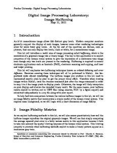
Color Fundamentals • Visible light is composed of a relatively narrow brand of frequencies in the electromagnetic spectrum. • If the light is achromatic (void of color), its only attribute is its intensity, or amount. • Achromatic light is what viewers see on a black and white television set. • Chromatic light spans the electromagnetic spectrum from approximately 400 to 700 nm.
© 2002 R. C. Gonzalez & R. E. Woods
Digital Image Processing, 2nd ed.
© 2002 R. C. Gonzalez & R. E. Woods
www.imageprocessingbook.com
Digital Image Processing, 2nd ed.
www.imageprocessingbook.com
Color Fundamentals • Three basic quantities are used to describe the quality of a chromatic light source: radiance, luminance, and brightness. – Radiance is the total amount of energy that flow from the light source, and it is usually measured in watts (W). – Luminance, measured in lumens (lm), gives a measure of the amount of energy an observer perceives from a light source. – Brightness is a subjective descriptor that is practically impossible to measure. It embodies the achromatic notion of intensity and is one of the key factors in describing color sensation. © 2002 R. C. Gonzalez & R. E. Woods
Digital Image Processing, 2nd ed.
www.imageprocessingbook.com
Color Fundamentals • 6 to 7 million cones in the human eye can divided into three principal sensing categories, corresponding roughly to red, green, and blue. • Approximately 65% of all cones are sensitive to red light, 33% are sensitive to green light, and only about 2% are sensitive to blue (but that blue cones are the most sensitive). • Due to these absorption characteristics of the human eyes, colors are seen as variable combinations of the so-called primary colors red (R), green (G), and blue (B). © 2002 R. C. Gonzalez & R. E. Woods
Digital Image Processing, 2nd ed.
www.imageprocessingbook.com
Color Fundamentals • It is important to keep in mind that having three specific primary color wavelengths for the purpose of standardization does not mean that these three fixed RGB components acting alone can generate all spectrum colors.
© 2002 R. C. Gonzalez & R. E. Woods
Digital Image Processing, 2nd ed.
© 2002 R. C. Gonzalez & R. E. Woods
www.imageprocessingbook.com
Digital Image Processing, 2nd ed.
www.imageprocessingbook.com
Color Fundamentals • The primary colors can be added to produce the secondary colors of light - magenta (red plus blue), cyan (green plus blue), and yellow (red plus green).
© 2002 R. C. Gonzalez & R. E. Woods
Digital Image Processing, 2nd ed.
© 2002 R. C. Gonzalez & R. E. Woods
www.imageprocessingbook.com
Digital Image Processing, 2nd ed.
www.imageprocessingbook.com
Color Fundamentals • The characteristics generally used to distinguish one color from another are brightness, hue, and saturation. • Hue is an attribute associated with the dominant wavelength in a mixture of light waves. • Hue represent dominant color as perceived by an observer. • Saturation refers to the relatives purity or the amount of white light mixed with a hue. © 2002 R. C. Gonzalez & R. E. Woods
Digital Image Processing, 2nd ed.
www.imageprocessingbook.com
Color Fundamentals • The pure spectrum color are fully saturation. • Hue and saturation taken together are called chromaticity, and therefore, a color may be characterized by its brightness and chromaticity.
© 2002 R. C. Gonzalez & R. E. Woods
Digital Image Processing, 2nd ed.
www.imageprocessingbook.com
Color Fundamentals • CIE chromaticity diagram (Fig 6.5), which show color composition as a function of x (red) and y (green). • For any value of x and y, the corresponding value of z (blue) is obtained from Eq.(6.1-4) by noting that z=1-(x+y). x = X (6.1 − 1) X +Y + Z Y (6.1 − 2) y= X +Y + Z Z (6.1 − 3) z= X +Y + Z (6.1 − 4) x + y + z =1
© 2002 R. C. Gonzalez & R. E. Woods
Digital Image Processing, 2nd ed.
Color Fundamentals
© 2002 R. C. Gonzalez & R. E. Woods
www.imageprocessingbook.com
Digital Image Processing, 2nd ed.
www.imageprocessingbook.com
Color Fundamentals • Any point not actually on the boundary but within the diagram represents some mixture o spectrum colors. • A straight-line segment joining any two points in the diagram defines all the different color variations that can be obtained by combining these two colors additively.
© 2002 R. C. Gonzalez & R. E. Woods
Digital Image Processing, 2nd ed.
www.imageprocessingbook.com
Color Fundamentals • The triangle in Figure 6.6 shows a typical range of colors (called the color gamut) produced by RGB monitors. • The irregular region inside the triangle is representative of the color gamut of today’s highquality color printing devices. • The boundary of the color printing gamut is irregular because color printing is a combination of additive and subtractive color mixing, a process that is much more difficult to control than that of displaying colors on a monitor. © 2002 R. C. Gonzalez & R. E. Woods
Digital Image Processing, 2nd ed.
Color Fundamentals
© 2002 R. C. Gonzalez & R. E. Woods
www.imageprocessingbook.com
Digital Image Processing, 2nd ed.
www.imageprocessingbook.com
Color Models • RGB (red, green, blue) model for color monitors and a board class of color video cameras. • CMY (cyan, magenta, yellow) and CMYK (cyan, magenta, yellow, black) models for color printing. • HIS (hue, saturation, intensity) model, which corresponds closely with the way humans describe and interpret color. • The HIS model also has the advantage that it decouples the color and gray-scale information in an image, making it suitable for many of the gray-scale techniques. © 2002 R. C. Gonzalez & R. E. Woods
Digital Image Processing, 2nd ed.
www.imageprocessingbook.com
The RGB Color Model • RGB image in which each of the red, green, and blue images is an 8-bit image. • The term full-color image is used often to denote a 24-bit RGB color image.
© 2002 R. C. Gonzalez & R. E. Woods
Digital Image Processing, 2nd ed.
www.imageprocessingbook.com
The RGB Color Model
© 2002 R. C. Gonzalez & R. E. Woods
Digital Image Processing, 2nd ed.
www.imageprocessingbook.com
The RGB Color Model • Many systems in use today are limited to 256 colors. • On the assumption that 256 colors is the minimum number of colors that can be reproduced faithfully by any system in which desired result is likely to be displayed. • Leaving only 216 colors that are common to systems. © 2002 R. C. Gonzalez & R. E. Woods
Digital Image Processing, 2nd ed.
Chapter 6 Color Image Processing
© 2002 R. C. Gonzalez & R. E. Woods
www.imageprocessingbook.com
Digital Image Processing, 2nd ed.
Chapter 6 Color Image Processing
© 2002 R. C. Gonzalez & R. E. Woods
www.imageprocessingbook.com
Digital Image Processing, 2nd ed.
www.imageprocessingbook.com
The CMY and CMYK Color Models • Where, again, the assumption is that all color values have been normalized to the range [0,1]. ⎡ C ⎤ ⎡1⎤ ⎡ R ⎤ ⎢ M ⎥ = ⎢1⎥ − ⎢G ⎥ ⎢ ⎥ ⎢⎥ ⎢ ⎥ ⎢⎣ Y ⎥⎦ ⎢⎣1⎥⎦ ⎢⎣ B ⎥⎦
© 2002 R. C. Gonzalez & R. E. Woods
Digital Image Processing, 2nd ed.
www.imageprocessingbook.com
The HIS Color Model • When humans view a color object, we describe it by its hue, saturation, and brightness. • Whereas saturation gives a measure of the degree to which a pure color is diluted by white light. • Brightness is a subjective descriptor that is practically impossible to measure. • It embodies the achromatic notion of intensity and is one of the key factors in describing color sensation. © 2002 R. C. Gonzalez & R. E. Woods
Digital Image Processing, 2nd ed.
Chapter 6 Color Image Processing
© 2002 R. C. Gonzalez & R. E. Woods
www.imageprocessingbook.com
Digital Image Processing, 2nd ed.
Chapter 6 Color Image Processing
© 2002 R. C. Gonzalez & R. E. Woods
www.imageprocessingbook.com
Digital Image Processing, 2nd ed.
Chapter 6 Color Image Processing
© 2002 R. C. Gonzalez & R. E. Woods
www.imageprocessingbook.com
Digital Image Processing, 2nd ed.
www.imageprocessingbook.com
Converting colors from RGB to HSI ⎧ θ H =⎨ ⎩360 − θ
if B ≤ G if B > G
1 ⎧ ⎫ ( ) ( ) [ ] − + − R G R B ⎪ ⎪ 2 θ = cos −1 ⎨ 1 ⎬ 2 ⎪ (R − G ) + (R − B )(G − B ) 2 ⎪ ⎩ ⎭
[
S = 1−
3 [min(R, G, B )] (R + G + B )
1 I = (R + G + B ) 3
© 2002 R. C. Gonzalez & R. E. Woods
]
It is assumed that the RGB values have been normalized to the range [0,1]
Digital Image Processing, 2nd ed.
www.imageprocessingbook.com
Converting colors from HSI to RGB RG sector (0o ≤ H < 120o )
GB sector(120o ≤ H < 240o )
B = I (1 − S )
H = H − 120o R = I (1 − S )
⎡ S cos H ⎤ R = I ⎢1 + ⎥ o − cos 60 H ⎣ ⎦ G = 1 − (R + B )
(
)
(
BR sector(240o ≤ H ≤ 360o ) H = H − 240o G = I (1 − S ) ⎡ S cos H ⎤ B = I ⎢1 + ⎥ o cos 60 H − ⎣ ⎦ R = 1 − (G + B )
(
© 2002 R. C. Gonzalez & R. E. Woods
⎡ S cos H ⎤ G = I ⎢1 + ⎥ o − H cos 60 ⎣ ⎦ B = 1 − (R + G )
)
)
Digital Image Processing, 2nd ed.
Chapter 6 Color Image Processing
© 2002 R. C. Gonzalez & R. E. Woods
www.imageprocessingbook.com
Digital Image Processing, 2nd ed.
Chapter 6 Color Image Processing
© 2002 R. C. Gonzalez & R. E. Woods
www.imageprocessingbook.com
Digital Image Processing, 2nd ed.
Chapter 6 Color Image Processing
© 2002 R. C. Gonzalez & R. E. Woods
www.imageprocessingbook.com
Digital Image Processing, 2nd ed.
Chapter 6 Color Image Processing
© 2002 R. C. Gonzalez & R. E. Woods
www.imageprocessingbook.com
Digital Image Processing, 2nd ed.
Chapter 6 Color Image Processing
© 2002 R. C. Gonzalez & R. E. Woods
www.imageprocessingbook.com
Digital Image Processing, 2nd ed.
Chapter 6 Color Image Processing
© 2002 R. C. Gonzalez & R. E. Woods
www.imageprocessingbook.com
Digital Image Processing, 2nd ed.
Chapter 6 Color Image Processing
© 2002 R. C. Gonzalez & R. E. Woods
www.imageprocessingbook.com
Digital Image Processing, 2nd ed.
Chapter 6 Color Image Processing
© 2002 R. C. Gonzalez & R. E. Woods
www.imageprocessingbook.com
Digital Image Processing, 2nd ed.
Chapter 6 Color Image Processing
© 2002 R. C. Gonzalez & R. E. Woods
www.imageprocessingbook.com
Digital Image Processing, 2nd ed.
Chapter 6 Color Image Processing
© 2002 R. C. Gonzalez & R. E. Woods
www.imageprocessingbook.com
Digital Image Processing, 2nd ed.
Chapter 6 Color Image Processing
© 2002 R. C. Gonzalez & R. E. Woods
www.imageprocessingbook.com
Digital Image Processing, 2nd ed.
Chapter 6 Color Image Processing
© 2002 R. C. Gonzalez & R. E. Woods
www.imageprocessingbook.com
Digital Image Processing, 2nd ed.
Chapter 6 Color Image Processing
© 2002 R. C. Gonzalez & R. E. Woods
www.imageprocessingbook.com
Digital Image Processing, 2nd ed.
Chapter 6 Color Image Processing
© 2002 R. C. Gonzalez & R. E. Woods
www.imageprocessingbook.com
Digital Image Processing, 2nd ed.
Chapter 6 Color Image Processing
© 2002 R. C. Gonzalez & R. E. Woods
www.imageprocessingbook.com
Digital Image Processing, 2nd ed.
www.imageprocessingbook.com
Color Transformations Formulation g ( x, y ) = T [ f ( x, y )] • The pixel value here are triplets or quartets. si = Ti (r1 , r2 , K , rn ), i = 1,2, K , n (6.5 − 2)
• {T1 , T2 ,K, Tn } is a set of transformation or color mapping functions that operate on ri to produce si . • If the RGB color space is selected, for example, n=3 and r1 , r2 , and r3 denote the red, green, and blue components of the input image. © 2002 R. C. Gonzalez & R. E. Woods
Digital Image Processing, 2nd ed.
www.imageprocessingbook.com
Color Transformations Formulation • Any of the color space components in Fig 6.30 can be used in conjunction with Eq.(6.5-2). • In theory, any transformation can be performed in any color model. • In practice, however, some operations are better suited to specific models.
© 2002 R. C. Gonzalez & R. E. Woods
Digital Image Processing, 2nd ed.
www.imageprocessingbook.com
Color Transformations Formulation • Suppose, for example, that we wish to modify the intensity of the image in Fig 6.30(a) using g ( x, y ) = kf ( x, y )
• In the HIS color space, this can be done with the simple transformation s3 = kr3
where s1 = r1 and s2 = r2
• Only HSI intensity component r3 is modified.
© 2002 R. C. Gonzalez & R. E. Woods
Digital Image Processing, 2nd ed.
www.imageprocessingbook.com
Color Transformations Formulation • In the RGB color space, three components must be transformed: si = kri i = 1,2,3. • The CMY space requires a similar set of linear transformations: si = kri + (1 − k ) i = 1,2,3.
© 2002 R. C. Gonzalez & R. E. Woods
Digital Image Processing, 2nd ed.
Chapter 6 Color Image Processing
© 2002 R. C. Gonzalez & R. E. Woods
www.imageprocessingbook.com
Digital Image Processing, 2nd ed.
Chapter 6 Color Image Processing
© 2002 R. C. Gonzalez & R. E. Woods
www.imageprocessingbook.com
Digital Image Processing, 2nd ed.
Chapter 6 Color Image Processing
© 2002 R. C. Gonzalez & R. E. Woods
www.imageprocessingbook.com
Digital Image Processing, 2nd ed.
Chapter 6 Color Image Processing
© 2002 R. C. Gonzalez & R. E. Woods
www.imageprocessingbook.com
Digital Image Processing, 2nd ed.
Chapter 6 Color Image Processing
© 2002 R. C. Gonzalez & R. E. Woods
www.imageprocessingbook.com
Digital Image Processing, 2nd ed.
www.imageprocessingbook.com
Tone and Color Corrections • A device-independent color model • The success of this approach is a function of the quality of the color profiles used to map each device to the model and the model itself. • The model of choice for many color management system (CMS) is the CIE L*a*b model.
© 2002 R. C. Gonzalez & R. E. Woods
Digital Image Processing, 2nd ed.
www.imageprocessingbook.com
Tone and Color Corrections ⎛Y ⎞ L* = 116 ⋅ h⎜⎜ ⎟⎟ − 16 ⎝ Yw ⎠ ⎡ ⎛ X ⎞ ⎛ Y ⎞⎤ ⎟⎟ − h⎜⎜ ⎟⎟⎥ a* = 500 ⎢h⎜⎜ ⎣ ⎝ X w ⎠ ⎝ Yw ⎠⎦ ⎡ ⎛ Y ⎞ ⎛ Z ⎞⎤ ⎟⎟⎥ b* = 200 ⎢h⎜⎜ ⎟⎟ − h⎜⎜ ⎣ ⎝ Yw ⎠ ⎝ Z w ⎠⎦ where 3 q ⎧⎪ q > 0.008856 h(q ) = ⎨ 16 ⎪⎩7.787 q + 116 q ≤ 0.008856
X w , Yw , and Z w are reference white tristimulus values © 2002 R. C. Gonzalez & R. E. Woods
Digital Image Processing, 2nd ed.
www.imageprocessingbook.com
Tone and Color Corrections • Like the HIS system, the L*a*b system is an excellent decoupler of intensity (represented by lightness L*) and color (represent by a* for red minus green and b* for green minus blue). • The tonal range of an image, also called its key type, refer to its general distribution of color intensities. • Most of the information in high-key images are located predominantly at low intensities; middle-key images lie in between.
© 2002 R. C. Gonzalez & R. E. Woods
Digital Image Processing, 2nd ed.
www.imageprocessingbook.com
Example 6.9 • Transformations for modifying image tones normally are selected interactively. • The idea is to adjust experimentally the image’s brightness and contrast to provide maximum detail over a suitable range of intensities. • In the RGB and CMY(K) spaces, this means all three (or four) color components with the same transformation function; in the HSI color space, only the intensity component is modified. • The S-shaped curve in the first row of the figure is detail for boosting contrast.
© 2002 R. C. Gonzalez & R. E. Woods
Digital Image Processing, 2nd ed.
Chapter 6 Color Image Processing
© 2002 R. C. Gonzalez & R. E. Woods
www.imageprocessingbook.com
Digital Image Processing, 2nd ed.
Chapter 6 Color Image Processing
© 2002 R. C. Gonzalez & R. E. Woods
www.imageprocessingbook.com
Digital Image Processing, 2nd ed.
www.imageprocessingbook.com
Histogram Processing • Histogram processing transformations of Section 3.3 can be applied to color images in an automated way. • As might be expected, it is generally unwise to histogram equalize the component of a color image independently. • This results in erroneous color. • A more logical approach is to spread the color intensities uniformly, leaving the colors themselves (e.g., hues) unchanged. • The HSI color space is ideally suited to this type of approach. © 2002 R. C. Gonzalez & R. E. Woods
Digital Image Processing, 2nd ed.
Chapter 6 Color Image Processing
© 2002 R. C. Gonzalez & R. E. Woods
www.imageprocessingbook.com
Digital Image Processing, 2nd ed.
www.imageprocessingbook.com
Smoothing and Sharpening Color Image Smoothing 1 c ( x, y ) = K
∑) c(x, y )
( x , y ∈S xy
⎡1 ⎤ R( x, y )⎥ ⎢ ∑ ⎢ K ( x , y )∈S xy ⎥ ⎢1 ⎥ c ( x, y ) = ⎢ G ( x, y )⎥ ∑ ⎢ K ( x , y )∈S xy ⎥ ⎢1 ⎥ ⎢ K ∑ B( x, y )⎥ ⎣ ( x , y )∈S xy ⎦ Thus, we conclude that smoothing by neighborhood averaging can be carried out on a per-color-plane basis. © 2002 R. C. Gonzalez & R. E. Woods
Digital Image Processing, 2nd ed.
www.imageprocessingbook.com
Example 6.12 • HSI color model is that it decouples intensity (closely related to gray scale) and color information, • This makes it suitable for many gray-scale processing techniques and suggests that is might be more efficient to smooth only the intensity component of the HSI representation.
© 2002 R. C. Gonzalez & R. E. Woods
Digital Image Processing, 2nd ed.
Chapter 6 Color Image Processing
© 2002 R. C. Gonzalez & R. E. Woods
www.imageprocessingbook.com
Digital Image Processing, 2nd ed.
Chapter 6 Color Image Processing
© 2002 R. C. Gonzalez & R. E. Woods
www.imageprocessingbook.com
Digital Image Processing, 2nd ed.
Chapter 6 Color Image Processing
© 2002 R. C. Gonzalez & R. E. Woods
www.imageprocessingbook.com
Digital Image Processing, 2nd ed.
www.imageprocessingbook.com
Color Image Sharpening ⎡∇ R( x, y )⎤ ⎢ 2 ⎥ 2 ∇ [c( x, y )] = ⎢∇ G ( x, y )⎥ ⎢∇ 2 B( x, y )⎥ ⎣ ⎦ 2
© 2002 R. C. Gonzalez & R. E. Woods
Digital Image Processing, 2nd ed.
Chapter 6 Color Image Processing
© 2002 R. C. Gonzalez & R. E. Woods
www.imageprocessingbook.com
Digital Image Processing, 2nd ed.
Color Segmentation • Segmentation in HSI color space • Segmentation in RGB Vector Space • Color Edge Detection
© 2002 R. C. Gonzalez & R. E. Woods
www.imageprocessingbook.com
Digital Image Processing, 2nd ed.
Chapter 6 Color Image Processing
© 2002 R. C. Gonzalez & R. E. Woods
www.imageprocessingbook.com
Digital Image Processing, 2nd ed.
www.imageprocessingbook.com
Segmentation in RGB Vector Space D(z, a ) = z − a
[ = [( z
]
= (z − a ) (z − a )
© 2002 R. C. Gonzalez & R. E. Woods
T
2
]
1 2 2
− aR ) + ( zG − aG ) + ( z B − a B ) 2
R
1 2
Digital Image Processing, 2nd ed.
Chapter 6 Color Image Processing
© 2002 R. C. Gonzalez & R. E. Woods
www.imageprocessingbook.com
Digital Image Processing, 2nd ed.
Chapter 6 Color Image Processing
© 2002 R. C. Gonzalez & R. E. Woods
www.imageprocessingbook.com
Digital Image Processing, 2nd ed.
Color Edge Detection ∂R ∂G ∂B r+ g+ b ∂x ∂x ∂x ∂B ∂G ∂R b g+ r+ v= ∂y ∂y ∂y
u=
∂R ∂G ∂B g xx = u ⋅ u = u T u = + + ∂x ∂x ∂x 2
2
2
2
∂R ∂G ∂B g yy = v ⋅ v = vT v = + + ∂y ∂y ∂y g xy = u ⋅ v = u T v =
© 2002 R. C. Gonzalez & R. E. Woods
2
2
∂R ∂R ∂G ∂G ∂B ∂B + + ∂x ∂y ∂x ∂y ∂x ∂y
www.imageprocessingbook.com
Digital Image Processing, 2nd ed.
www.imageprocessingbook.com
Color Edge Detection The direction of maximum rate of change of c(x,y) is given by this angle ⎡ 2 g xy ⎤ 1 −1 θ = tan ⎢ ⎥ 2 ⎢⎣ (g xx − g yy )⎥⎦
rate of change at (x,y), in the direction of θ , is given by
[
]
⎧1 ⎫ F (θ ) = ⎨ (g xx + g yy ) + (g xx − g yy )cos 2θ + 2 xy sin 2θ ⎬ ⎩2 ⎭
© 2002 R. C. Gonzalez & R. E. Woods
1 2
Digital Image Processing, 2nd ed.
Chapter 6 Color Image Processing
© 2002 R. C. Gonzalez & R. E. Woods
www.imageprocessingbook.com
Digital Image Processing, 2nd ed.
Chapter 6 Color Image Processing
© 2002 R. C. Gonzalez & R. E. Woods
www.imageprocessingbook.com
Digital Image Processing, 2nd ed.
Chapter 6 Color Image Processing
© 2002 R. C. Gonzalez & R. E. Woods
www.imageprocessingbook.com
Digital Image Processing, 2nd ed.
www.imageprocessingbook.com
Noise in Color Images • In cases when, say, only one RGB channel is affected by noise, conversation to HSI spreads the noise to all HSI component images.
© 2002 R. C. Gonzalez & R. E. Woods
Digital Image Processing, 2nd ed.
Chapter 6 Color Image Processing
© 2002 R. C. Gonzalez & R. E. Woods
www.imageprocessingbook.com
Digital Image Processing, 2nd ed.
Chapter 6 Color Image Processing
© 2002 R. C. Gonzalez & R. E. Woods
www.imageprocessingbook.com
Digital Image Processing, 2nd ed.
Chapter 6 Color Image Processing
© 2002 R. C. Gonzalez & R. E. Woods
www.imageprocessingbook.com
Digital Image Processing, 2nd ed.
Chapter 6 Color Image Processing
© 2002 R. C. Gonzalez & R. E. Woods
www.imageprocessingbook.com