Eur. Phys. J. B 10, 263–270 (1999)

THE EUROPEAN PHYSICAL JOURNAL B EDP Sciences c Societ`

a Italiana di Fisica Springer-Verlag 1999

Diffraction by finite-size crystalline bundles of single wall nanotubes S. Rols1,2 , R. Almairac1 , L. Henrard1 , E. Anglaret1,a , and J.-L. Sauvajol1 1 2

Groupe de Dynamique des Phases Condens´eesb , Universit´e Montpellier II, 34095 Montpellier Cedex 5, France Institut Laue-Langevin, 38042 Grenoble Cedex, France Received 16 December 1998 Abstract. We calculate the diffraction spectrum of finite-size crystalline bundles of single wall carbon nanotubes (SWNT). The general profile of the spectrum as well as the width and position of the (1 0) diffraction peaks of the 2-D lattice of bundles depend on the tubes symmetry, distribution of tubes diameters and diameter of the bundles. Consequently, any attempt to derive the mean-diameter of the tubes from a diffraction spectrum requires to consider the diameters distribution of the tubes and the size of the bundles. Experimental diffraction profiles of various single wall nanotubes samples are well fitted by the calculated spectra. PACS. 61.12.Bt Theories of diffraction and scattering – 61.10.Dp Theories of diffraction and scattering – 61.46.+w Clusters, nanoparticles, and nanocrystalline materials

1 Introduction Single-wall carbon nanotubes (SWNT) are promising systems for basic science in one-dimension and nanoapplications in electronics. Some of their physical properties, including mechanical, elastic, transport, are known to depend on their molecular structure, helical pitch, and bundle-like crystalline packing [1]. Transmission electronic microscopy (TEM) observations have shown that the SWNT usually self-assemblate to form finite-size crystalline-like bundles of some tens to some hundreds tubes [2,3]. TEM [2–4], electron diffraction [5] and Raman [3,6–8] investigations have shown that in most of the cases a sample contains various kinds of nanotubes, i.e. tubes of various diameters and symmetries. The diffraction profile of the crystalline ropes of SWNT has been previously reported and modelised assuming a 2-D infinite hexagonal lattice of uniform cylinders [2,3,9,11]. Thess et al. used an arbitrary line width to account for the peak broadening due to the finite diameter of the bundles [2]. Such an approach is not relevant for polydisperse samples, as illustrated by the disagreement found between the mean tube diameter derived from TEM measurements and from the position of the diffraction peaks in reference [9], and discussed elsewhere [10]. In a recent work, Rinzler et al. fitted their experimental data with a series of Gaussian lines in order to get an estimate of the tube diameter distribution [11]. None of these former analysis took properly into account a b

e-mail: [email protected] CNRS UMR 5581

both the finite size of the crystalline ropes and the tube diameter distribution. In the present work, we compute the diffraction spectra for SWNT bundles formed with a finite number of tubes and consider various distributions of tube diameters. Our model is presented in Section 2. Section 3 deals with the general changes in the spectra related to the variation of the structural parameters of the samples, i.e. the symmetry of the tubes, the mean tube diameter and polydispersity, the diameter of the bundles. The width and position dependences of the most intense (1 0) Bragg peak with respect to the structural parameters of the ropes are presented and discussed in Section 4. In Section 5, we report experimental diffraction measurements on SWNT and fit them with calculated spectra. From the fit, we derive a structural picture of the samples. We conclude in Section 6.

2 Principles of the calculations 2.1 Numerical samples The SWNT were built by rolling up graphene sheets to form tubes with various diameters and symmetries. Following the usual terminology of reference [1], we hereafter use the pair of integers (n, m) to refer to the rolling up vector and distinguish the following helicities: armchair (n, n), zigzag (n, 0) and chiral (n, m 6= n). Tubes with diameters Dt ranging from 6.7 to 30 ˚ A were considered. The nanotubes were placed parallel one to each others on a finite-size 2D hexagonal array of cell parameter a0 = Dt +dt−t to form concentric shells, with an intertube

264

The European Physical Journal B

˚ value slightly smaller than spacing dt−t fixed to 3.2 A, the inter-graphene sheets distance in graphite, in agreement with calculations [12] and experiments [2]. Calculations were carried out for bundles of various diameters Db , (hereafter, we call Nt the number of tubes per bundle). The spectrum for a polydisperse sample is the sum of the spectra calculated for each of the bundles forming the sample, which were prepared in the following way: the distribution of tubes diameters D was chosen to fit a Gaussian distribution N (D) ∝ exp [−(

D − Dt 2 )] σt

Z'

rs Z

r0

rc

M (X, Y, Z)

rs,t

Y'

O2

X' rt

r rproj

(1)

Y O1

X

centered on Dt with a standard deviation σt (the full width at half √ maximum of the distribution is therefore FWHM = 2 ln 2σt ). For large polydispersities, the Gauss function was truncated below 6.7 ˚ A and above 30 ˚ A in order to keep reasonable values for the tubes diameters. We recall that most of the experimental observations by electronic microscopy show that the bundles are made of nanotubes with a rather small diameter dispersity [2–4]. By contrast, the mean-diameter of the tubes is found to depend on the area of investigation [3] (this probably relates to the temperature of the growth area). Therefore, we built each bundle with a set of monodisperse SWNT of diameter D (D varies from a bundle to another). We assumed that Nt was a constant for all bundles so that we got a double source of polydispersity: that on the tubes diameters fixed by σt and that on the bundles diameters fixed by Nt and D. However, as discussed below, we checked that the profile of the spectra and in particular that of the (1 0) peak depends essentially on the tubes diameters dispersity and is sensitive to the size of the bundle only for small Nt .

O2 R2,3

rt r0

O1

O3

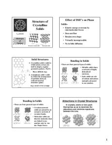
Fig. 1. Schematic representation of the system of coordinates and variables used for the calculations.

where the integration is made on the surface of the sphere of radius |Q|. The density of atom nuclei writes as follows (Fig. 1): ρ(r) ∝

Ns Nt X X

δ 3 (r − rs,t )

(4)

t=1 s=1

2.2 Expression of the diffraction cross section The model used for calculating the powder diffraction spectra is based on the general formulas for X-rays/ neutrons diffraction [13]. In the case we are dealing with (elastic and coherent diffraction), the intensity of the wave diffracted by one bundle writes as follows: Z I(Q) ∝ || fs exp(iQ · r)ρ(r)d3 r||2 (2) volume

where Q is the scattering vector, ρ(r) is the density of scatterers in the sample and fs is the atomic scattering amplitude of the scatterer s (fs is a function of Q for Xrays while this is a constant, the atomic scattering length, for neutrons). In a powder experiment, the diffraction is to be averaged on all the directions of space or, equivalently, on all the orientations of the scattering vector in the reciprocal space. The mean diffracted intensity thus writes: RR I(Q)d2 Q hI(Q)i ∝ (3) 4πQ2

where rs,t is the position of scatterer s on tube t. As far as one considers static scatterers, the intensity calculated using equations (1) to (3) has to be modulated by the Debye-Waller factor exp(−2W (Q)), where W = 12 hQ2 u2 i and hu2 i are the mean-square vibrational amplitudes of the atoms. For the computation, we used the values of hu2 i of graphite [14]. The expression of I(Q) thus writes (Fig. 1): hI(Q)i ∝ exp(−2W (Q)) Z π/2 Z × dθ sin(θ) 0

π

dφ|s(Q)S(Q)F (Q)|2 (5) 0

PNs where F (Q) = s=1 fs exp(iQrs ) is the structure factor of the nanotube unit cell i.e. the smallest periodic unit PN c along z, s(Q) = c ) is the intratube interc=1 exp(iQr P Nt ference function and S(Q) = t=1 exp(iQrt ) is the intertube interference function. The index s, c and t refer to the scatterers, tubes unit cells and tubes, respectively (Fig. 1), and Ns , Nc and Nt are the number of scatterers in an unit cell, the number of unit cells in a tube and the number of tubes in a bundle, respectively. The atomic position thus writes r = rt + rc + rs .

S. Rols et al.: Diffraction by finite-size crystalline bundles of single wall nanotubes

˚−1 ) of the spectra is senThe high-Q range (Q > 2 A sitive to the intrinsic structure of individual tubes. It was calculated using equations (3, 4) and considering each atom nucleus on each tube as a scatterer. This allows to calculate rigorously neutron diffraction spectra. Calculation of the peaks intensities of X-rays diffraction spectra would require a more sophisticated choice of the position of the scatterers since one should describe accurately the electronic densities on the folded graphene sheets. By contrast, the low-Q part of the diffraction pattern (below Q = 2 ˚ A−1 ) is only sensitive to the crystalline order in the bundle and its calculation doesn’t require to consider the discrete position of each scatterer on the tubes. In this low-Q range, we assumed an infinite length for the tubes and considered the following uniform density of scatterers at the surfaces of the tubes, relevant for calculating both X-rays and neutron diffraction spectra: ρ(r) ∝

Nt X

δ(|rt − rproj | − r0 )

(6)

t=1

where r0 is the radius of the tubes and rproj is the projection of r on the (XY ) plane (Fig. 1). Using equation (2), one gets: hI(Q)i ∝ exp(−2W (Q))

Nt X r0 2 J0 (Ri,j Q) P (Q) Q i,j=1

(7)

where P (Q) ∝ [fs J0 (r0 Q)]2 is the form factor of one tube (plotted in Fig. 2a), J0 is the zero order Bessel function and Ri,j is the distance between tubes i and j in the bundle.

3 Qualitative features of the diffraction spectra In this section, we are interested in characteristic features of the diffraction spectra and changes associated with the variations of each structural parameter. Figure 2 presents the calculated diffraction spectra for various sets of parameters. We first deal with the tube helicity-dependent features of the spectra. Figure 2a presents some diffraction spectra calculated for bundles formed by SWNT of comparable diameter but various helical pitches. As expected, only the high-Q range is sensitive to intratubes density correlations. The spectra all superimpose below 2 ˚ A−1 but present a specific profile above. The diffraction pattern for chiral tubes is much more complex because of their lower symmetry, and consequently the larger size of the unit cell. Therefore, high resolution diffraction measurements should allow to discuss the symmetry of SWNT and provide an averaged “bulk” information by contrast with the local one derived from electronic diffraction investigations [5]. Such signatures are however unlikely to be experimentally measured because of the weakness of the signal in this Q range, the wide distribution of helical pitches of SWNT in most of the samples, and the

265

intense contribution of the diffraction peaks of graphite and residual catalysts in the same Q-range. At low-Q, the diffraction profile is sensitive to the structure of the bundles, i.e. to their diameter and to the diameter dispersity of the tubes. As expected, the general profiles of the spectra are similar to those calculated for an infinite hexagonal array of tubes [2], except at very lowQ where some additional peaks are found (see below the (1 0) peak in Fig. 2). These are signatures of the finite-size of the bundles and correspond to diffraction lines for which extinctions rules are canceled because of the finite number of diffraction planes. The position of these peaks depends on the diameter of the tubes Dt (Fig. 2b), the diameter of the bundles Db (Fig. 2c) and the standard deviation of the Gaussian distribution σt (Fig. 2d). As Db → ∞, these peaks vanish and one recovers as expected the regular spectrum of an infinite crystal (not shown). The broadening of the diffraction lines can also prevent their observation. This occurs for samples with large polydispersities (Fig. 2d). In experimental studies, not only the polydispersity of the samples can prevent the observation of these peaks, but also the lack of resolution as well as the small angle scattering signal from porosity and impurities. The apparent positions of the diffraction peaks Q(hk) , where h and k are the Miller index, are shifted with respect to the Bragg positions Q∞ (hk) for an infinite network of monodisperse tubes because of the modulation of the diffraction pattern by the SWNT form factor. Thess et al. already discussed this effect [2] but used arbitrary lineshapes to account for it in their calculations. Figure 2 shows that the width of the diffraction peaks depends significantly both on the bundle diameter (Fig. 2c), as expected for periodic structures of finite-size and in a larger extent on the polydispersity (even for a small one, see Fig. 2d). As expected, the broader the peaks (finite-size effects or polydispersity) and the larger the difference between Q∞ (hk) and the maximum of the form factor, the larger the shift of the diffraction peaks with respect to Q∞ (hk) and the smaller their intensity. The broadening of the (1 0) peak and the concomitant shift will be discussed in detail in the next section. Consequently, any attempt to derive a mean-tube diameter from the position of the peaks should take into account the diameter of the bundle and the polydispersity of the sample. Actually, as illustrated in Figure 2, a careful study of the diffraction spectra not only allows to derive the mean-tube diameter but provides an estimate of their diameter dispersity and of the diameter of the bundles. This explains the systematic disagreement between Dt estimated from TEM experiments and from the position of the diffraction peaks [10], that was reported in reference [9]. In the purpose of being useful for the analysis of experimental spectra, we propose in the next section a detailed quantitative analysis of the width and position of the most intense of the diffraction peaks, the (1 0) peak, which provides the most characteristic signature of the bundle-like packing. We report in Section 5 original neutron diffraction measurements on samples prepared by the arc electric technique and by laser ablation

266

The European Physical Journal B

Fig. 2. Left part of the figure: schematic representation of the samples: a) the different helicities of the nanotubes, b) and c) a bundle, d) the diameter distribution of the tubes. Right part of the figure: diffraction spectra of bundles of SWNT for various sets of structural parameters. Dt is the mean tube diameter, Db the diameter of a bundle, Nt the number of tubes in a bundle and σt the standard deviation of the Gaussian distribution. a) Dt ' 13.6 ˚ A, Nt = 19, σt = 0, various helical pitches (armchair A (6,6), 13.6 ˚ A (10,10), 19.0 ˚ A (14,14)), (10,10), zigzag (17,0) and chiral (15,5)); b) Armchair SWNT with various Dt (8.1 ˚ A ((10,10) SWNT), various Nt (7, 91, 721), σt = 0; d) Dt = 13.6 ˚ A ((10,10) SWNT), Nt = 37, Nt = 37, σt = 0; c) Dt = 13.6 ˚ A, 6 ˚ A). Spectra in (a) were calculated using the discrete positions of each scatterer. The form factor of one various σt (0, 3 ˚ tube, whose intensity has been multiplied by an arbitrary factor for clarity, is superimposed with the diffraction spectra in (b).

S. Rols et al.: Diffraction by finite-size crystalline bundles of single wall nanotubes

0.2

0.2

a) Nt = 7

∆Q (10) (Å-1)

∆ Q (10)(Å-1 )

N t = 91

0.1

0.05

0 5

b) D t = 8.1 Å

N t = 37

0.15

267

D t = 13.7 Å

0.15

D t = 19 Å

0.1

0.05

10

15

20

25

0

30

50

100 150 200 250 300 350 400

D t (Å)

D b (Å) 0.4

c)

-1 ∆ Q (10)(Å )

0.35 0.3 0.25 0.2 0.15 0.1 0.05 0 0

2

4

6

σ (Å) t

8

10

12

Fig. 3. Dependence of the width of the (1 0) Bragg peak of the bundles over the following structural parameters: a) tubes diameter (for various bundles diameters and σt = 0); b) diameter of the bundle (for various tubes diameter and σt = 0); c) A and Nt = 37). tubes diameters distribution (for Dt = 13.6 ˚

that can only be fitted by considering a small and significant polydispersity, respectively.

4 Quantitative analysis of the (1 0) peak In Figures 3 and 4, we plot the width (FWHM) ∆Q(10) and apparent position Q(10) dependences of the (1 0) diffraction peak as a function of (a) the diameter of the tubes, (b) the diameter of the bundle and (c) the standard deviation of the Gaussian distribution of the tubes diameters. Let’s first discuss the width of the peak. For monodisperse samples (same tubes, same bundles), ∆Q(10) is found to increase when the tubes diameters decrease and/or the number of tubes per bundle decreases (Fig. 3a). Actually, we find that the width only depends on the diameter of the bundle, independently of the diameter of the tubes inside (Fig. 3b), as expected for periodic structures of finite size. On the other hand, the width of the peak increases when the diameter dispersity of the tubes increases (Fig. 3c). This is the expected signature in

the reciprocal space of the coexistence of nanocrystallites (bundles) with various cell parameters in the sample. The position of the peak is also found to depend on all these parameters: the mean-tube diameter, the diameter of the bundles and the tubes diameters dispersity (Fig. 4). As expected, Q(10) increases when Dt decreases. In addition, Q(10) increases when the number of tubes per bundle decreases (Fig. 4a). A significant shift to high Q is actually observed only for very small bundles (Db < 200 ˚ A, see Fig. 4b). The product Q(10) a0 , proportional to the ratio between the position of the peak in a finite network and that in an infinite one, Q(10) /Q∞ (10) , is found to depend only on the diameter of the bundle for σt = 0 independently of the tubes diameters, as illustrated by the mastercurve plotted √ in Figure 4b. As expected, one recovers Q∞ (10) ' 4π/( 3a0 ) for large bundles of monodisperse tubes (dashed line in Fig. 4b). By contrast, a huge shift to low-Q is systematically observed for polydisperse samples and the smaller the tubes, the larger the shift (Fig. 4c). As a tool for experimenters, we report in the inset

268

The European Physical Journal B

8.5

0.8

b)

a)

D t = 8.1 Å

Nt=7

0.7

Nt=37

D t = 19 Å

Q (10).a0

Q(10) (Å-1)

0.6

D t = 13.7 Å

8.0

Nt=91

0.5

7.5

0.4 0.3

7.0 0

0.2 5

10

15

20

25

30

D t( Å )

50 100 150 200 250 300 350 400

D b (Å)

Fig. 4. Dependence of the position of the (1 0) Bragg peak of the bundles over the following structural parameters: a) cell parameter of the bundle (for various number of tubes per bundle and σt = 0); b) product Q(10) a0 over the diameter of the ˚ bundle (for various tubes diameters and σt = 0), where a0 = Dt + √3.2 A is the cell parameter of the bundle. The dashed line corresponds to the limit expected for infinite networks Q∞ ' 4π/ 3a ; 0 c) tubes diameters distribution (for various mean-tube (10) diameters and Nt = 19); inset: product Q(10) a0 .

of Figure 4c the product Q(10) a0 as a function of σt for three values of Dt . From a mean-value of the tubes diameter derived from microscopic or spectroscopic experiments, one can estimate with a rather good accuracy the tubes diameter dispersity from these data as long as the dispersity is significant (and therefore the shift due to dispersity larger than that due to the finite-size of the bundles) [10]. However, a rigorous analysis of the data also requires to consider the general profile of the diffraction spectra, as discussed in the next section. The peculiar broadening and shift of the (1 0) peak all have a same origin, i.e. the modulation of the Bragg pattern by the form factor of the nanotubes. For an infinite and homogeneous crystal, the diffraction peaks are Dirac peaks and the form factor only modulates their intensity. As soon as the reflections get an intrinsic nonzero width, the modulation by the form factor leads in addition to some variations of the position and width of the peaks. This occurs because of the difference be-

tween the position of the peaks and the extrema of the form factor (Fig. 2b, see also Fig. 2 in reference [2]). The apparent position and intensity of the (1 0) peak depend both on its intrinsic √ width and on the relative positions of Q∞ (10) = 4π/( 3a0 ) and the first extrema of the form factor, i.e. Qmin ' 4.8/Dt and Qmax ' 7.6/Dt for the first minimum and maximum, respectively. Let’s call R the ratio (Qmax − Q(10) )/(Qmax − Qmin ). R tends to zero when Dt increases and increases up to the unity when Dt decreases down to ' 6.3 ˚ A, a diameter slightly smaller than the smallest nanotube diameter allowed [1]. Consequently, one finds that the intensity of the Q(10) peak continuously increases for increasing tubes diameters while it vanishes when Dt decreases. Therefore, when one deals with polydisperse samples, the diffraction spectrum is dominated by the contribution of large tubes. This leads to a shift to low-Q of Q(10) and to a concomitant overestimation of the mean-tube diameter [9]. For a distribution of diameters centered on that of (10,10) SWNT and a standard

S. Rols et al.: Diffraction by finite-size crystalline bundles of single wall nanotubes

269

linewidth of the SWNT peaks, and close to that of the (0 0 2) graphite peak (located around 1.87 ˚ A−1 in Fig. 5). Two series of samples were investigated. The first one was prepared by the electric arc discharge (EA) technique at Montpellier using an experimental set-up presented in detail in reference [3]. Other samples were synthesized by an original laser ablation (LA) technique (significantly different than that of the Rice group [2]) in Zaragoza, as described in reference [4]. A detailed investigation of the structure of the nanotubes in these samples will be presented elsewhere [15]. The exact position and shape of the (1 0) peak as well as those of the other peaks obviously depend on the synthesis parameters (chemical nature and amount of catalysts used, nature and pressure of the gas filling the reactive chamber...). However, the general features of the diffraction spectra appear to be above all technique-dependent. Rather narrow peaks are recorded for EA samples with the (1 0) peak pointing out between 0.40 and 0.45 ˚ A−1 . The general profile of the spectra is rather similar to that reported by Thess et al. [2] for samples prepared by laser ablation by the Rice group. By contrast, the diffraction profiles for the LA samples from Zaragoza present broader linewidths and the (1 0) peak points out between 0.30 and 0.35 ˚ A−1 . Typical spectra are presented in Figures 5a and 5b, respectively. The hypothesis of larger mean tube diameters to the LA profile was in disagreement with TEM observations that allow to estimate a mean-diameter very close to that observed for EA samples [4]. The TEM observations also indicate that the mean-diameter of the bundle is rather similar for the EA and LA samples, with a number of tubes per bundle usually found to lie between 30 and 50. However, by contrast with EA samples, the general broad profile of the spectra for LA samples is the first signature of a significant polydispersity and the TEM observations do confirm the presence of some large tubes in small but significant amount [4]. Fig. 5. Comparison between experimental and calculated diffraction spectra. a) electric arc sample (details in the text) fitted with Dt = 13.6 ˚ A, Nt = 37, σt = 2 ˚ A. In the intermediate curve, a polynomial background has been subtracted from the experimental data; b) laser ablation sample (details in the A, Nt = 37, σt = 6 ˚ A. text) fitted with Dt = 13.6 ˚

deviation σt = 4 ˚ A, the overestimation of Dt is about 10% and increases up to 40% for σt = 8 ˚ A(Fig. 4c).

5 Fits of experimental data We present in Figure 5 experimental neutron diffraction (ND) spectra recorded on the spectrometer G6-1 at Laboratoire L´eon Brillouin, Saclay, France. The spectra were measured at room temperature using an incident wavelength λ = 4.73 ˚ A and corrected for the empty cell background and the sensibility of the detectors. The resolution was checked to be much smaller than the intrinsic

Therefore we fitted the data with spectra calculated with the following fixed parameters: Dt = 13.7 ˚ A and Nt = 37 and various σt . The best agreement with the data was found for σ = 2 ˚ A and σ = 6 ˚ A for the EA and LA spectrum, respectively (see solid lines in Fig. 5). We emphasize that for a number of tubes in the bundles larger than 30, the calculated spectrum almost doesn’t depend on Nt (see Fig. 4b) and therefore an accurate value of Nt can not be derived from the fit. The agreement is observed both for the position and shape of the (1 0) peak and the general profile of the spectra. However, in the EA case, a poor agreement was found in the low-Q range where the calculation didn’t reproduce well the huge increase of intensity below 0.3 ˚ A−1 . We point out that in this low-Q range, one expects both an intrinsic contribution from the form factor of the tubes and a possible additional contribution from the scattering of nanoparticles of catalysts or of other carboneous species. For the EA samples, the shoulder around 1.84 ˚ A−1 on the left part of the (0 0 2) graphite peak is assigned to graphite nanoparticles. A peak at the same position is recorded for multiwall carbon nanotubes (MWNT) [16] but we checked

270

The European Physical Journal B

by electron microscopy that no MWNT were observable in these samples [3]. In addition, we recorded the diffraction signature of a significant amount of Ni catalysts particles (not shown). On the other hand, the intrinsic contribution to low-Q scattering from the nanotubes is expected to be small because of the narrow distribution of tubes diameters. This explains the disagreement between experiment and calculations in the low-Q range. If one subtracts a polynomial background from the spectrum, one recovers a good agreement above 0.3 ˚ A−1 (see Fig. 5a). Note that the intensity of the higher order peaks is slightly weaker in the experiments. This might be assigned to some fluctuations of the lattice constant due to tube diameter dispersity within a single bundle that was not considered in our calculations and that would increase the width of the higher order peaks. By contrast, in the LA case, only a very small amount of impurities can be detected form the diffraction spectra. In addition, one expects rather large low-Q signal because of the presence of small tubes (see Fig. 2). For these samples, the agreement between experiment and calculations is good all over the Q-range, including the low-Q part.

6 Conclusion A classical approach for the calculation of the diffraction spectra of bundles of single wall carbon nanotubes was developed. The effect of the mean-tube diameter, the finitesize of the bundles and the diameter dispersity of the tubes on the general profile and the particular position and linewidth of the (1 0) peak were discussed. We find that the width and apparent position of the peak is significantly dependent on all the structural parameters above. This explains the systematic overestimation of the tube diameter with respect to TEM analysis reported in the literature [9,10]. A good agreement between experiments and calculations is found for samples prepared both by the arc electric discharge technique in Montpellier and an original laser ablation technique developed in Zaragoza. The distribution of tubes diameters is found to be rather narrow for the EA samples and more polydisperse for the LA samples. A detailed Raman investigation on similar samples that corroborates the present results will be published elsewhere [15]. We thank I. Mirebeau for her help in the neutron diffraction experiments and the Laboratoire L´eon Brillouin, Saclay, France for providing beamtime on their neutron facilities. We acknowl-

edge C. Journet and P. Bernier, as well as W.K. Maser, E. Mu˜ noz, A.M. Benito, M.T. Martinez and G.F. de la Fuente for providing high-quality samples. One of us (S.R.) acknowledges financial support from the R´egion Languedoc-Roussillon.

References 1. M.S. Dresselhaus, G. Dresselhaus, P.C. Eklund, Science of fullerenes and carbon nanotubes (Academic Press, New-York, 1996). 2. A. Thess, R. Jee, P. Nikolaev, H. Dai, P. Petit, J. Robert, C. Xu, Y. Hee Lee, S. Gon Kim, A.G. Rinzler, D.T. Colbert, G.E. Scuseria, D. Tomanek, J.E. Fischer, R.E. Smalley, Science 273, 483 (1996). 3. C. Journet, W.K. Maser, P. Bernier, A. Loiseau, M. Lamy de la Chapelle, S. Lefrant, P. Deniard, R. Lee, J.E. Fischer, Nature 388, 756 (1997). 4. W.K. Maser, E. Munoz, A.M. Benito, M.T. Martinez, G.F. de la Fuente, Y. Maniette, E. Anglaret, J.L. Sauvajol, Chem. Phys. Lett. 292, 587 (1998). 5. J.M. Cowley, P. Nikolaev, A. Thess, R.E. Smalley, Chem. Phys. Lett. 265, 379 (1997); L. Henrard, A. Loiseau, C. Journet, P. Bernier (to be published). 6. A.M. Rao, E. Richter, S. Bandow, B. Chase, P.C. Eklund, K.A. Williams, S. Fang, K.R. Subbaswamy, M. Menon, A. Thess, R.E. Smalley, G. Dresselhaus, M.S. Dresselhaus, Science 275, 187 (1997). 7. A. Kasuya, Y. Sasaki, Y. Saito, K. Tohji, Y. Nishina, Phys. Rev. Lett. 78, 4434 (1997). 8. E. Anglaret, N. Bendiab, T. Guillard, C. Journet, G. Flamant, D. Laplaze, P. Bernier, J.L. Sauvajol, Carbon 36, 1815 (1998). 9. S. Bandow, S. Asaka, Y. Saito, A.M. Rao, L. Grigorian, E. Richter, P.C. Eklund, Phys. Rev. Lett. 80, 5003 (1998). 10. E. Anglaret, S. Rols, J.L. Sauvajol, Phys. Rev. Lett. 81, 4780 (1998). 11. A.G. Rinzler, J. Liu, H. Dai, P. Nikolaev, C.B. Huffman, F.J. Rodriguez-Macias, P.J. Boul, A.H. Lu, D. Heymann, D.T. Colbert, R.S. Lee, J.E. Fischer, A.M. Rao, P.C. Eklund, R.E. Smalley, Appl. Phys. Lett. A 67, 29 (1998). 12. J.C. Charlier, X. Gonze, J.P. Michenaud, Europhys. Lett. 29, 43 (1995). 13. S.W. Lovesey, Theory of neutron scattering from condensed matter (Oxford Sciences, 1984). 14. R. Almairac (unpublished results). 15. S. Rols, E. Anglaret, J.L. Sauvajol, G. Coddens, A.J. Dianoux, Appl. Phys. A (to be published); J.L. Sauvajol et al., Phys. Rev. B (submitted). 16. O. Zhou, R.M. Fleming, D.W. Murphy, C.H. Chen, R.C. Haddon, S.H. Glarum, Science 263, 1744 (1994).