Determination of forward & futures prices Chapter 3 Exercises and Assignments
Exercise 1:
Proving the futures price formula n
Show by an arbitrage argument that the futures price formulae just provided are correct:
F0 = S0 (1 + r )T F0 = S0 erT
Copyright © 2002, Robert Cressy
−S 0
F0 > S 0e
Answer rT
Borrow S
Buy Stock
Short Future NCF
CF 0
CFT
S0
− S0 e
− S0 0 0
F0 < S 0 e r T rT
0
Lend S
Sell Stock short
CF0
− S0 S0
(Sell Stock)
F0 F0 − S 0e r T > 0
CFT
S 0 erT 0 (Buy Stock)
Long Future NCF
0 0
− F0 S0e r T −F0 > 0
Copyright © 2002, Robert Cressy
1
n
Using the above table note that n
If the futures price deviates from the formula arbitrage is always possible n
If F 0 > S0 e rT then the futures price is too high relative to the spot or cash price n
Then short the future and buy spot
n
The spot purchase will be used to close out the futures position rT This locks in a certain gain of F 0 − S 0e > 0
n
n
If F 0 < S 0 e rT then the futures price is too low relative to the spot n n n
Hence take a long position in the future and short the spot The short sale means is used to close out the futures position This locks in a certain gain of S 0 e rT − F0 > 0
Copyright © 2002, Robert Cressy
Exercise 2
Value of a forward contract n
Use an arbitrage argument to prove the formulae for the value of long and short forward contracts (assuming continuous compounding): ƒ = ( F0 – K )e–rT g =(K – F0 )e–rT
Copyright © 2002, Robert Cressy
Value of a long forward K PAST
CF -t
Enter long forward in gold for delivery at price K=100
0
NOW
1
LATER
CF T
0
Buy gold under long contract at K=100
-100=-K
2
Sell gold under short contract at F0=150
3 Enter short forward contract at current delivery price F0=150
NCF:
CF 0
(F 0 − K) e−rT = (150 − 100 )e− 0. 1 = 45.24
4
150=F0
F0 − K = 150−100 = 50
Copyright © 2002, Robert Cressy
2
Answer n
We consider only the long forward contract (K) here. n
Consider a contract to buy n n
1 oz gold on 1 January 2004 (12 months time) at price of $100
n
This contract was entered into on 1 July 2002 (6 months ago)
n
Currently (1 Jan 2003) a forward contract for Jan 2004 gold in 1 year is $150/oz The annual interest rate (cont. comp.) is 10%
n
n
Hence there are 12 months left to run
Copyright © 2002, Robert Cressy
Answer cont’d If in 1 year (1 Jan 2004) I were to n n
n
Buy 1 oz gold at the delivery price of $100 and Then to sell the 1 oz at $150
Then I would pocket a profit of n
-$100+$150=$50/oz
Copyright © 2002, Robert Cressy
Answer cont’d n
n
n
This means I short the current futures contract with delivery price $150 in 1 year
So: How much would I pay now for the forward contract with delivery price of $100? Clearly, given the opportunity cost, I would pay p.d.v. of (Current delivery price – historical delivery price) I.e. $(150-100)e -0.1x1 = $50e -0.1x1 =$45.24
Copyright © 2002, Robert Cressy
3
Answer cont’d n
Generalising this we have the value of a long forward contract: p.d.v. of (Current delivery price – historical delivery price) I.e. f = (F0-K)e -rT
Copyright © 2002, Robert Cressy
Exercise 3: Stock index futures n
Using the data from Wall Street Journal (see next slide) n
n
Calculate the average r-q for the S&P 500 index.
Assume the current value of the index is 112,900 n
What is the price of a 3 month futures contract on the S&P 500?
Copyright © 2002, Robert Cressy
Data Stock index futures: Price calculation from S&P data CONTRACT DATE SETTLEMENT PRICE % CHANGE Sep-98 107,400.00 Dec-98 108,550.00 Mar-99 109,650.00 Jun-99 110,780.00 AVERAGE r-q = Current value of S&P: 112,900.00 3 month futures price:
Copyright © 2002, Robert Cressy
4
Answer n
We use the formula:
n
Where r is a rate per annum T = years With T=0.75 ST=110,780 S0=107,400 we get
S 0 e( r− q ) T = S T ⇒ r − q = ln(S T / S 0 ) / T n n
r − q = ln(110, 780 / 107, 400) / 0.75 = 0. 04131 = 4.131% p.a. Copyright © 2002, Robert Cressy
n
Then to calculate the price of a 3 month futures contract on the S&P 500 as: T = 0 .25 , r = 0 .04131 F3 = (112,900)e0 .04131x 0. 25 x price per unito f index = 114,072. 15x price per unito f index
Copyright © 2002, Robert Cressy
Exercise 4:
Transactions costs and arbitrage n
n
We assume in the above arbitrage argument zero transactions costs Is this important? Explain.
Copyright © 2002, Robert Cressy
5
Answer There are 500 stocks in the S&P index for example Arbitrage involving the purchase of 500 stocks could be
n n
n n
expensive in terms of commission Time-consuming to arrange
It is potentially important for the argument to be valid
n
n
However, complex trades are now automated and performed by computers.
Copyright © 2002, Robert Cressy
Exercise 5: n
Show that the relation between u and U is given by S0 + U = S 0e uT
Copyright © 2002, Robert Cressy
n
This is a one liner: F0 = S 0 e( r +u ) T = ( S0 + U )e rT
#
⇒ S 0 euT = S 0 +U
Copyright © 2002, Robert Cressy
6
Assignment 1:
Arbitrage with transactions costs n n
A trader owns silver as part of a long term investment portfolio He can n n
n
Buy silver @ $250/oz Sell silver @ $249/oz
He can also Borrow @ 6% pa Lend @ 5.5% pa. (both with annual compounding) n n
Copyright © 2002, Robert Cressy
Assgn’t 3 cont’d n
n
What is the range of 1-year forward prices of silver that precludes arbitrage? Generalise this to show that as the differences disappear prices converge on the equilibrium price rT F0 = S0 e
where S0 = 249.5 (say) and r = 0.0575 (say) (Assume no bid-offer spread in forward prices). Copyright © 2002, Robert Cressy
−S 0
Answer Originally: no transactions costs F0 > S 0e
rT
Borrow S
Buy Stock
Short Future NCF
CF 0
CFT
S0
− S0 e
− S0 0 0
F0 < S 0 e r T rT
0
CF0
S 0 erT
Sell Stock short
S0
0
Long Future
0
(Sell Stock)
F0 F0 − S 0e r T > 0
CFT
− S0
Lend S
(Buy S)
NCF
0
− F0 S0e r T −F0 > 0
Copyright © 2002, Robert Cressy
7
With transactions costs F0 > S 0e
rT
Borrow S
Buy S
CF0
CFT
S0 B = 250
− S0B er T
− S0 B = −250
0
Short F
0
NCF
F0 < S 0 e r T Lend S
= − 250e0.06 Sell S short
0
CF0
S 0 S er T
= −249
= 249e0.055
S 0S = 249
(Sell S)
(Buy S)
F0 F0 − 250 e
CFT
− S 0S
Long F
0 .06
NCF
0 0
− F0 . 249e 0055 − F0
Copyright © 2002, Robert Cressy
Answer cont’d n
Hence arbitrage is possible if F0 > 250e0. 06 = 265.46
n
Or if F0 < 249e0. 055 = 263.08
n
The no-arbitrage condition is therefore 265.46 > F0 > 263. 08 Copyright © 2002, Robert Cressy
Interpretation n
With differences either in n n
buying and selling prices or borrowing and lending rates
we find that: there is a range of forward prices in which no arbitrage is possible n within this range there is no tendency for prices to change n
Copyright © 2002, Robert Cressy
8
n
As these differences get smaller n
Forward prices converge on the equilibrium value:
F0 = S0 e rT n
At this value there is no room for arbitrage
Copyright © 2002, Robert Cressy
9