FAU-PI1-DISS-07-001
Design studies for the KM3NeT Neutrino Telescope
Den Naturwissenschaftlichen Fakult¨aten der Friedrich-Alexander-Universit¨at Erlangen-N¨ urnberg zur Erlangung des Doktorgrades
vorgelegt von Sebastian Kuch aus N¨ urnberg
Als Dissertation genehmigt von den Naturwissenschaftlichen Fakult¨aten der Universit¨at Erlangen-N¨ urnberg.
Tag der m¨ undlichen Pr¨ ufung:
18. Juli 2007
Vorsitzender der Pr¨ ufungskomission:
Prof. Dr. Eberhard B¨ansch
Erstberichterstatter:
Prof. Dr. Ulrich F. Katz
Zweitberichterstatter:
Prof. Dr. Els DeWolf
Zusammenfassung Die Entdeckung der kosmischen Strahlung durch Viktor Hess 1912 markiert den Beginn der Astroteilchenphysik. Das Ziel dieser Disziplin ist die Erforschung kosmischer Ph¨anomene durch die Detektion von kosmischen Teilchen auf der Erde. Dies beginnt bei den Protonen und leichten Kernen der kosmischen Strahlung selbst, die in Luftschauerexperimenten nachgewiesen werden. Diese Experimente liefern Informationen u ¨ ber die Zusammensetzung und das Energiespektrum der kosmischen Strahlung. Sie konnten jedoch bis jetzt keine Informationen u ¨ber den Ursprung ihrer hochenergetischen Teilchen liefern, da diese geladen sind und, außer bei den h¨ochsten Energien (E > 1019 eV) durch das galaktische Magnetfeld abgelenkt werden, wodurch sie ihre Richtungsinformation verlieren. Vielversprechender ist hier das Neutrino, das mangels Ladung nicht in elektromagnetischen Feldern abgelenkt wird. Da Neutrinos nur schwach wechselwirken, werden sie im interstellaren Medium oder kosmischen Staubwolken kaum absorbiert. Weiterhin erlauben Neutrinos dem Beobachter ins Zentrum von heissen und dichten Objekten zu blicken, die f¨ ur elektromagnetische Strahlung undurchl¨assig sind. Wenn ein Objekt Protonen auf die Energien der kosmischen Strahlung beschleunigt wechselwirken diese mit der Materie oder der Strahlung um das Objekt, wobei u ¨ ber Zwischenschritte geladene Pionen erzeugt werden, bei deren Zerfall Myon- und Elektron-Neutrinos entstehen. Die Entdeckung von kosmischen Neutrinoquellen k¨ame also der Entdeckung des Ursprungs der kosmischen Strahlung gleich. Es gibt viele Kandidaten f¨ ur solche individuellen Quellen hochenergetischer (E > 1 GeV) kosmischer Neutrinos, wie z.B. Aktive Galaktische ¨ Kerne, Supernova-Uberreste oder sogenannte Gamma-Ray-Bursts, die auch Kandidaten f¨ ur Quellen der kosmischen Strahlung sind. Die gleichen Eigenschaften, die das Neutrino zu einem idealen Botenteilchen f¨ ur die Astroteilchenphysik machen, erschweren seine Detektion. Durch den sehr geringen Wirkungsquerschnitt werden riesige Targetvolumina ben¨otigt. F¨ ur Neutrinoteleskope werden deshalb nat¨ urliche Volumina wie das Wasser in der Tiefsee und das antarktische Eis instrumentiert. Interagiert ein Neutrino mit den Nukleonen des Targetmaterials, so entstehen geladene Sekund¨arteilchen, die sich mit einer Geschwindigkeit bewegen, die gr¨osser ist als die Lichtgeschwindigkeit im Detektormedium. Deshalb senden diese Teilchen CherenkovPhotonen aus, die Hilfe von Lichtsensoren (Photomultipliern, PMn) detektiert werden. Aus den Ankunftszeiten und Amplituden der Photonen-Treffer in den PMn kann die Richtung und die Energie des einfallenden Neutrinos rekonstruiert werden. Ein Neutrinoteleskop ist also im wesentlichen eine dreidimensionale Anordung von Photosensoren. Die Signatur einer Neutrinoreaktion im Detektor h¨angt vom Neutrino-flavour ab. Am bedeutendsten sind hierbei Myon-Neutrinos, die bei ihrer Wechselwirkung (geladener Strom)
II Myonen erzeugen (und einen hadronischen Schauer). Myonen haben in Wasser und Eis eine sehr große Reichweite (> 1 km f¨ ur E > 1 TeV) und erzeugen lange Spuren von Cherenkov-Licht, was eine Rekonstruktion der Richtung erleichtert. Die große Reichweite erm¨oglicht auch die Detektion von Myonen, die weit außerhalb des Detektorvolumens erzeugt wurden. Andererseits ist die Energierekonstruktion schwierig, da unbekannt ist welcher Teil der Myonenspur ausserhalb des Detektors verlief. Bei den Wechselwirkungen von Elektron- und Tau-Neutrinos, sowie bei allen Wechselwirkungen u ¨ ber den neutralen Strom entstehen hadronische und elektromagnetsiche Schauer, die ihre Energie schnell an das Medium verlieren und deshalb Reichweiten von nur etwa 10 m haben. Dies erschwert die Richtungsrekonstruktion. F¨ ur Schauer im Innern des Detektorvolumens ist allerdings die Energierekonstruktion einfacher, da die gesamte Energie des Schauers im Detektor deponiert wird. Weltweit sind einige Neutrinoteleskope im Betrieb oder im Aufbau. Am S¨ udpol befindet sich das AMANDA-Teleskop das schon seit Ende der neunziger Jahre Daten nimmt. Im russischen Baikal-See befindet sich das Baikal-Experiment, das erste funktionierende Wasser-Neutrinoteleskop. Im Mittelmeer ist das ANTARES-Experiment im Aufbau vor der s¨ udfranz¨osischen K¨ uste und wird 2007 fertiggestellt sein. Das griechische NESTORProjekt hat bereits erfolgreich Prototypen getestet und mit ihnen erste Daten genommen. Diese Experimente demonstrieren die Funktionalit¨at der Technolgie von Neutrinoteleskopen in der Tiefsee (oder dem tiefen Eis). Dennoch ist bereits jetzt absehbar, das die Volumina dieser Teleskope zu klein sind, um das volle Potential der Neutrinoastronomie auszusch¨opfen. Detektoren mit einem intrumentierten Volumen von (mindestens) einem Kubikkilometer werden dazu n¨otig sein. Am S¨ udpol hat der Bau des Nachfolgers des AMANDA-Teleskops, des IceCube Detektors, bereits begonnen. Im Mittelmeer betreibt das italienische NEMO-Projekt seit einiger Zeit Vorstudien f¨ ur ein Kubikkilometer-Teleskop. Da Neutrino-Teleskope die Erde als Abschirmung gegen atmosph¨arischen Untergrund (Myonen aus Luftschauern) ben¨otigen, sind zwei Teleskope notwendig, um den gesamten Himmel abzudecken, eines auf der Nord- und eines auf der S¨ udhalbkugel. Der schnelle Fortschritt des IceCube-Projekts legt die Zeitskala f¨ ur ein Kubikkilometer-Experiment auf der Nordhalbkugel fest. Deshalb haben sich die europ¨aischen Neutrino Teleskop-Experimente ANTARES, NEMO und NESTOR zusammengeschlossen mit dem Ziel einer Designstudie f¨ ur ein Kubikkilometer-Neutrinoteleskop im Mittelmeer, dem KM3NeT-Projekt. Diese Designstudie erfordert zun¨achst intensive Simulationen zur Optimierung des Detektordesigns. Da bis jetzt keine dedizierte KM3NeT-Software existiert und der Zeitplan der Designstudie knapp ist, wurde in dieser Arbeit die ANTARES-Software verwendet. Die NEMO-Kollaboration verwendet diese Software bereits seit einiger Zeit f¨ ur die Simulation des NEMO Detektor-Konzepts, was ihre Anwendbarkeit auf gr¨oßere Geometrien beweist. Die ANTARES- Simulationskette enth¨alt im Prinzip alle f¨ ur eine breite Studie n¨otigen Komponenten. Dies beginnt bei der Erzeugung eines Software-Modells des zu simulierenden Detektors. Dies besitzt im wesentlichen zwei Ebenen. Die kleinste Einheit ist das sogenannte Stockwerk, eine lokale Anordnung von PMn mit definierten Eigenschaften wie Richtung und Ort der Photomultiplier im Stockwerk, sowie deren technische Daten. Die zweite Ebene ist die Geometrie, also die Anordnung dieser Stockwerke im instrumentierten Volumen. Die technischen Details der Positionierung der Stockwerke, also die
III Frage ob sie an Kabeln (strings, ANTARES) oder semifesten T¨ urmen (towers, NEMO, NESTOR) in der Tiefsee verankert werden, wurden hier nicht betrachtet, da f¨ ur eine Absch¨atzung der Leistung eines Detektors zun¨achst nur die Positionen und Eigenschaften der PM relevant sind. Der n¨achste Schritt in der Simulationskette ist die Simulation der einfallenden Neutrinos und ihrer Wechselwirkungen im Medium. Die entstehenden geladenen Sekund¨arteilchen werden anschliessend zum bzw. durch den Detektor propagiert. Hier wird die Cherenkov- Lichterzeugung simuliert und die Antwort des Detektors in Form von Photon-Treffern in PMn (Zeiten und Amplituden) bestimmt. Aus den Treffern wird schließlich mit Hilfe eines Rekonstruktionsalgorithmus die Richtung des Neutrinos ¨ bestimmt. Die meisten dieser Komponenten sind mit geringen technischen Anderungen auf eine Vielzahl verschiedener Detektor-Konzepte anwendbar. Die einzige Ausnahme ¨ ist der Rekonstruktionsalgorithmus, der trotz einiger Anderungen, auf die ANTARESKonfiguration optimiert ist. Eine gleichartige Effizienz f¨ ur die verschiedenen untersuchten Detektor-Konfigurationen ist daher unwahrscheinlich. F¨ ur diese Studie wurden ausschliesslich Myon-Neutrinos im Energiebereich zwischen 10 GeV und 10 PeV simuliert. Dieser Energiebereich deckt das gesamte Spektrum der Physikziele von Neutrinoteleskopen ab. Beginnend bei der Suche nach Neutrinos aus den Annihilationen von dunkler Materie (WIMPs) in Schwerkraftzentren wie der Sonne (E < 1 TeV), u ¨ber die Suche nach individuellen Quellen kosmischer Neutrinos (1 TeV < E < 100 TeV), bis zur Suche nach Neutrinos aus dem diffusen Fluss aller kosmischen Neutrinoquellen (E > 100 TeV). Der optische Untergrund (aus 40 K-Zerf¨allen und Biolumineszenz) wurde mit einer Rate von 90.9 Hz pro cm2 Photokathodenfl¨ache simuliert (entspricht 40kHz pro 10PM). F¨ ur die u ¨brigen Umgebungsparameter wurden die ANTARES Standardwerte verwendet. Um die verschiedenen Detektor-Konfigurationen vergleichen zu k¨onnen, wurde die Effektive Neutrinofl¨ache berechnet, die ein Maß f¨ ur die Effizienz des Detektors ist und die einfache Berechnung von Ereignisraten f¨ ur gegebene Neutrinofl¨ usse erm¨oglicht. Weiterhin wurde die Winkelaufl¨osung bestimmt (der Median der Verteilung der Winkelabweichung zwischen ’wahrem’ Neutrino und rekonstruiertem Myon), was die Anwendung des Rekonstruktionsalgorithmus erfordert. Um m¨oglichst unab¨angig von der Rekonstruktion zu bleiben, wurde ein Satz von Kriterien definiert, der es erlaubt, das Potential eines Detektormodells einzusch¨atzen. Die wichtigsten sind das sogenannte minimal-Kriterium welches das absolute Minimum an Treffern in PMn verlangt, das f¨ ur eine Rekonstruktion der Myon-Spur n¨otig ist, das selected-Kriterium, das auf der Rekonstruktion basiert und das moderate-Kriterium das mindestens 6 (Signal-)Treffer in 6 verschiedenen Stockwerken verlangt. Ersteres ist die optimistischste (und wahrscheinlich unrealistischste) Option, das selected-Kriterium stellt den schlechtesten Fall dar, w¨ahrend die moderate-Bedingung die wahrscheinlich realistischste Absch¨atzung ist. Zun¨achst wurden verschiedene Photomultiplier-Konfigurationen untersucht. Im wesentlichen handelt es sich dabei um Anordnungen von drei verschiedenen PM-Typen. Der in ANTARES und AMANDA verwendete 10PM (Hamamatsu R7081-20), ein sehr viel kleinerer 3PM (Photonis XP53X2), der eine bessere Quanteneffizienz, einen kleineren Transit Time Spread (TTS) und bessere Photonseperation bietet, sowie ein 20PM. F¨ ur den Vergleich der verschiedenen Anordnungen (schematisch dargestellt in Abb. 1) wurden die jeweiligen Stockwerke in einem homogenen quaderf¨ormigen Gitter mit horizontalen
IV
b.) electronics
������� ������������������ ������� ������� ������������������ ������ ������ ������ ������ ������ ������ ������ ������ �������������� �������� �������� �������� �������� � ������ ������ ������ ������ ������ ���� ���� ���� ���� ���� ���� ���� ���� ���� ���� ���� ���� ���� ���� ���� ���� ���� ���� ��� ����� ����� ����� ���������� ����� ����� ����� ����� ����� ����� ����� ����� ����� ����� ����� ����� ��� ������������ ������ ������ ������ ������ ������ ������ ������ ������ ������ ������ ������ ������ ������ ������ ������ ���� ������ ��� ��� ��� ��� ��� ��� ��� ��� ��� ��� ��� ��� ��� ��� ��� ��
e.)
\ ]P \ ]P \ ]P \ ]P \ ]\ iP O QP O QP O QP O QP O QO ]P h iP h ih QP iP \ ]P \ ]P \ ]P \ ]\ hiP O QP O QP O QP O QP O QO ]\P]P h iP h ih QP iP \ ]P \ ]P \ ]P \ ]\ hiP O QP O QP O QP O QP O QO ]\P]P h iP h iP h ih QP \ \ \ \ \ O O O O O SRQO ]\P P ] P ] P ] P ] ] P Q P Q P Q P Q ^ _P ^ _P ^ _P ^ _^ kP R kjih SP R SP R SP R SP R SP RQP _^P_P h kP h kP h SP iP iP iP j j j ^ _P ^ _P ^ _P ^ _^ jP R R R R R R _^P_P P S P S P S P S P S P S SR P j P j j k k SP k SP ^ _P ^ _P ^ _P ^ _^ kkP R R R R R R _^P_P P S P S P S P S SR j kP j kP j SP kj R SP ^aP ^aP ^aP ^aP RUP RUP RUP _^P ` _P ` _P ` _P ` _^a` mP T mlkj SP T RUP T SP T SP T SP T SRUT a`P_P UP j mP j mP j RUP kP kP kP l l l ` aP ` aP ` aP ` a` mP T ml UP T UP T UP T UP T UP T UT a`PaP UP l l l P m P m ` aP ` aP ` aP ` a` mP T ml UP T UP T UP T UP T UP T UT a`PaP l mP l mP l UP `cP `cP `cP `cP TWP TWP TWP TWP TWP TWP a`P b aP b aP b aP b a`cb oP V onml UP V UP V UP V UP V UP V UTWV cbPaP l oP l oP l UP mP nmP nmP b cP b cP b cP b cb noP V on WP V WP V WP V WP V WP V WV cbPcP WP n n n P o P o b cP b cP b cP b cb nP V V V V V V WV cbPcP P W P W P W P W P W WP P n P n n o o WP o WP b eP b eP b eP b edcb ooP V YP V YP V YP V YXWV PeP dcP dcP dcP dcP XV qpon YP XV YP XWP XWP XWP XWP edcbP n qP n qP n YP oP oP p p p P q d eP d eP d eP d ed qP X qp YP X YP X YP X YP X YP X YX edPeP YP p p p P q P q d eP d eP d eP d ed qP X qp YP X YP X YP X YP X YP X YX edPeP YP p p p P q P q d gP d gP d gP d gfed qP X qp [P X [P X [P X [P X [P X [ZYX PgP feP feP feP feP ZYP ZYP ZYP ZYP ZYP ZYP gfedP p sP p sP p [P qP qP r r r r P s s f gP f gP f gP f gf sP Z sr [P Z [P Z [P Z [P Z [P Z [Z gfPgP [P r r r P s P s f gP f gP f gP f gf sP Z sr [P Z [P Z [P Z [P Z [P Z [Z gfPgP [P r r r P s P s f gP f gP f gP f gf rP Z rs [P Z [P Z [P Z [P Z [P Z [Z gfPgP s rP s rP s [P
� � � � � � � � � � � � � � � � � � � � � � � � � � � � � � � � � �
�� � � � � � � � � � � � � � � � � � � � � � � � � � � � � � � � �
� � � � � � � � � � � � � � � � � � � � � � � � � � � � � � � � � �
� � � � � � � � � � � � �� � � �� � � �� � � �� � � �� � � � � � � � � � � � � � � � ���� � ��� � ��� � ��� � ��� �� �� �� �� �� �� �
d.)
c.)
# $� # $# � $� � �� � �� � �� �� �� �� �� � �� # �� $#��� $� $# �� ��� �� �� � �� �� � �� �� � �� �� �� # ��� # ��� $� � �� � �� ���� �� � ���� �� � $� � $# �� � ���� � �� � �� � �� � �� ���� � �� � �� � �� � �� ���� � �� � �� � �� � �� ���� � �� � �� � �� � �� ���� � �� � �� � �� � �� ���� � �� � �� � �� � �� ���� � �� � �� � �� � �� ���� � �� � �� � �� � �� ���� � �� � �� � �� � �� ���� � �� � �� � �� � �� ���� � �� � �� � �� � �� � � � � � � �� � � � � � � � � � &% �� % &%�&� % �� &� � � � � � � � � � � � � � � &% �� � �� � �� % &� % �� �� &%�&� � � � � � � � � % &� % &% � &%�&� � � � � � � � � �
electronics
a.)
electronics
electronics ���������� ������ ������ ������ ���� ��� � � � � ����
����
����
����
����
����
������
����� ����
����� ����
����� ����
����� ����
��� ����
����
����
����
����
����
��
� �� ��� �� �� �� �� �� �� �� �� �� �� �� �� �� �� �� �� �� �� �� �� �� �� �� �� �� �� �� �� �� �� �� � �
�� � ��� �� �� �� �� �� �� �� �� �� �� �� �� �� �� �� �� �� �� �� �� �� �� �� �� �� �� �� �� �� �� �� � �
���
��� �� �� �� �� �� �� �� �� �� �� �� �� �� �� �� �� �� �� �� �� �� �� �� �� �� �� �� �� �� �� �� ��
f.)
: ;* : ;* : ;* : ;: 9*9*9*9*9 ;* : ;* : : ;* : ;: 9* 9* 98 8 9* 8 9* 8 ?* < =* < =* < =* < =* < ;* < ;: =< ;* =* : ;* : ;: 89* > ?* > ?* > ?* > ?> ;: =* ;* 9* 98 ?* 8 9* 8 9* 8 >?* * < =* < =* < =* < ;: =* < ;: =< ;* =* ? >* ? >* ? >? 98 >* 8 9* 8 9* 8 9* 8 ??* < =* < =* < =* < ;: =* < ;: =< ;* = > ?* > ?* > ?* > ?> * 9 * 9 * 9 9 ?* 8 8 8 8 ?* < 76 =* < 76 =* < 76 =* < 76 =* < 76 =* < =< > 88 ?* > A* > A* > A* > A* * ? * ? ?* @ @ @ @ ?> A* @ A@ 6*76*=* * 8 * 8 * 8 * 8 < 76 =* < 76 =* < 76 =* < 76 =* < 76 =* < =< > ?* > A* > A* > A* > A* ?* @ ?* @ ?* @ ?* @ ?> A* @ A@ 6*7* 6 =* @ A* @ A* @ A* @ A* @ A@ 6*7* 6 7* 6 7* 6 7* 6 7* 6 76 A* @ A* @ A* @ A* @ A* @ A@ 6*7* 6 7* 6 7* 6 7* 6 7* 6 76 A* 2 3* 2 3* 2 3* 2 3* 2 3* 2 32 , -* , -* , -* , -* , -, electronics 3* -* 2 3* 2 3* 2 3* 2 3* 2 3* 2 32 , -* , -* , -* , -* , -, 3* -* 2 5* 2 5* 2 5* 2 5* 2 54 3* 2 32 , +* 4 3* 4 3* 4 3* 4 3* 4 3* -* 5* ) -, +* ) -, +* ) -, +* ) -, +* ) -, +* ) +) 2 5* 2 5* 2 5* 2 5* 2 54 3* 2 32 , +* 4 3* 4 3* 4 3* 4 3* 4 3* -* ) -, +* ) -, +* ) -, +* ) -, +* ) .*-, +* ) /* . +)+) /* . /* . /. 1* 0 1* 0 1* 0 5* 4 1100 5* 4 5* 4 5* 4 5* 4 54 ) +* ) +* ) +* ) +* ) .*+* ) /* +* . /* . /. 1* 0 1* 0 1* 0 5* 4 10 5* 4 5* 4 5* 4 5* 4 54 ) +* ) +* ) +* ) +* ) .*+* ) ./* +* +) /* . /* . /. 1* 0 1* 0 1* 0 5* 4 10 5* 4 5* 4 5* 4 5* 4 54 5* ) +* ) +* ) +* ) +* ) .*+* ) ./* +* +) /* . . . . 0 0 0 * / * / / * 1 * 1 * 1 4 10 5* 4 5* 4 5* 4 5* 4 54 ) +* ) +* ) +* ) +* ) .*+* ) /* +* . +) /* . /* . /. 1* 0 1* 0 1* 0 5* .*/* . /* . /* . /. 1* 0 1* 0 1* 0 10
" �� !� " !" ���� � !� �� ! "! "! �� "� ���� �� �� ! ! "! " �� � � � ����� "�
� �� � (� �� ' �� (� ' (' � '� ����� ( �� '� ( '( ' (� ' (' (�
g.) electronics E FC E FC E FC E FC E FE FC E FC E FC E FC E FE FECFC E BC E BC E BC E BC FECBCFC D FC D FC D FC D FEE BC D BD E BC E BC E BC E BC FECBCFC BDHC D FC D FC D FC DGCF BC DHC G HC G HG BCBC D BC D BC D BC DGCBC DGHC G BBDDHC G HC G HG BCBC D BC D BC D BC DGCBC DGC H GC H GH BCBC BDGC D BC D BC D BC DGCBC DHHC G G HC G HG HC BCBC D BC D BC D BC DGCBC DHC G BDHC G HC G HG GCHC G HC G HC G HG
KCKC L KC L KC L KC L KC L KL KCLC K LC K LC K LC K LC K LK K NC K NC K NC K NM LC K LK MN KCNC M LC M LC M LC M LC C C K K K K K K LK M M M M M M C L C L C L C L LC C N C N C N C N C N N I JC I JIC JC JI NC M M M M M M C N C N C N C N N I JC I JIC JC JI NC M M M M M M C N C N C N C N N IC C I C I I J J J NC J NC M NC M NC M NC M NM I JC I MNC I JICJC J M NC M NC M NC M NM I JC I JC I M JI NC JC I JC I JI JICJC
Abbildung 1: Schematische Darstellung der simulierten Stockwerktypen. a.) Stockwerk mit einem einzelnen 10¨oder 20PM; b.) Stockwerk mit 2 10PMn; c.) ANTARES Stockwerk, 10¨oder 20PM; d.) Zwillings-ANTARES Stockwerk mit sechs 10PMn; e.) Multi-PM Zylinder-Stockwerk mit 36 3PMn; f.) Multi-PM Kugel-Stockwerk mit 36 oder 42 3PMn; g.) Multi-PM Kugel-Stockwerk mit 21 3PMn.
(string-) und vertikalen (Stockwerk-)abst¨anden von 63 m angeordnet. Das Volumen dieser Geometrie betr¨agt nahezu genau einen Kubikkilometer, der mit 4840 Stockwerken instrumentiert ist. Zus¨atzlich wurde f¨ ur alle Stockwerk-Typen die deutlich weniger oder mehr Photokathodenfl¨ache besitzen eine zus¨atzliche Geometrie erzeugt, wobei die Anzahl der Stockwerke pro ßtringßo angepaßt wurde, dass die gesamte Photokathodenfl¨ache einem Referenzdetektor entspricht. Diese Konfigurationen wurden candidate-Detektoren genannt. Dem zugrunde liegt die Annahme, dass die Kosten f¨ ur ein Neutrinoteleskop im wesentlichen proportional zur Photokathodenfl¨ache sind. Als Referenzstockwerk wurde das Standard ANTARES-Stockwerk verwendet. Wie zu erwarten, sind Detektoren mit gr¨oßerer Photokathodenfl¨ache im allgemeinen besser (mehr effektive Fl¨ache, bessere Winkelaufl¨osung). Detektoren mit nur einem PM pro Stockwerk verlieren bei der Rekonstruktion drastisch an Effizienz, da der Algorithmus unter anderem lokale Koinzidenzen ben¨otigt, also Treffer in mehreren PMn eines Stockwerkes innerhalb eines definierten Zeitfensters. Dies dient der Unterdr¨ uckung des optischen Untergrundes. bei einem Stockwerk mit einem einzelnen PM gibt es offensichtlich keine lokalen Koinzidenzen. Zwar k¨onnen auch Treffer mit Amplituden u ¨ber einer definierten Schwelle verwendet werden, doch ist deren Anzahl im Allgemeinen zu klein. Da lokale Koinzidenzen mit großer Wahrscheinlichkeit auch bei einer dedizierten KM3NeT-
V Rekonstruktionsstrategie verwendet werden, sind Stockwerke mit einzelnen PMn stark im Nachteil. Die Stockwerke mit 3PMn, 36 davon in verteilt auf drei Glaszylinder oder 42 bzw. 21 in einer Glasskugel pro Stockwerk, zeigen unter etwa 10 TeV zu niedrigen Energien deutlich ansteigende effektive Fl¨achen. Dies wird vor allen Dingen durch die h¨ohere Quanteneffizienz der PM verursacht. Die Winkelaufl¨osung ist ¨ahnlich wie f¨ ur die Stockwerke mit 10PMn. Besonders effizient scheint dabei die Version mit 21-PMKugelstockwerken. Durch die gr¨oßere Anzahl von Stockwerken pro string ist die hier die Instrumentierung dichter, was die Lichtausbeute verbessert. Dabei wurde die besseren Photonseparations-Eigenschaften der 3PMs in der Simulation noch nicht ber¨ ucksichtigt. Zwei Stockwerk-Konfigurationen wurden mit 20PMn best¨ uckt. Das erste entspricht dem ANTARES Stockwerk (also 3 20PMn), w¨ahrend das zweite einen einzelnen 20PM tr¨agt. Letzteres leidet unter den gleichen Nachteilen wie die Variante mit einzelnen 10PMn pro Stockwerk und liefert trotz h¨oherer Photokathodenfl¨ache als beim Referenzdetektor keine besseren Ergebnisse. Die erste Variante ist allen anderen Detektoren bei Energien unter 100 TeV u ucksichtigt werden, dass es sich nicht um eine ¨ berlegen. Es muss aber ber¨ ’candidate-Version’ handelt (die h¨atte nur zwei Stockwerke pro string, was ziemlich unrealistisch ist). Die Kosten f¨ ur einen derart ausgestatteten Detektor w¨aren also deutlich h¨oher (die 20PM sind teurer und erfordern gr¨oßere Druckbeh¨alter). Der Nutzen dieser Konfiguration h¨angt somit von den genauen Kosten ab. Um die verschiedenen Detektorgeometrien zu vergleichen, wurden die jeweiligen Detektormodelle mit den 36-PM-Zylinder-Stockwerken best¨ uckt. Einige Besipiele f¨ ur untersuchte Geometrien werden in Abb. 2 gezeigt. Zun¨achst wurden verschiedene ringf¨ormige Konfigurationen simuliert. Da die Reichweite von Myonen mit Energien u ¨ber 1 TeV in Wasser die Gr¨oßenordnung von 1 km (also in etwa die Dimension des Detektors) u ¨berschreitet, erreichen die meisten Myonen den Detektor von außerhalb. Daher ist bei diesen und h¨oheren Energien eine große Querschnittsfl¨ache wichtiger als ein großes instrumentiertes Volumen. Dieser Effekt k¨onnte genutzt werden, um die Anzahl an Strings (und damit Strukturen und Kosten) zu reduzieren. Ringgeometrien sind eine einfache M¨oglichkeit dieses Konzept umzusetzen. Die Anzahl der Strings wurde bei ann¨ahernd gleicher Anzahl von Stockwerken um mehr als ein Drittel reduziert. Die resultierenden effektiven Fl¨achen sind verglichen mit dem Quader bei niedrigen Energien aufgrund der dichteren Instrumentierung im Ring etwas besser, f¨ ur Energien u ¨ ber etwa einem TeV (abh¨angig vom verwendeten Kriterium) jedoch etwa 10% schlechter. Die Ursache f¨ ur die geringere Effizienz bei hohen Energien ist der Anteil von Myonen, der den Detektor nahezu vertikal passiert. Die Querschnittsfl¨ache ist f¨ ur solche Ereignisse aufgrund des Lochs¨ım Ring geringer. Bei gleicher Photokathodenfl¨ache scheinen die Ringe also gem¨aß der Annahme zu funktionieren. Bei einer Reduktion der Photokathodenfl¨ache nimmt die Effizienz jedoch drastisch ab. Das Konzept kann also eine geringere Anzahl von Stockwerken nicht kompensieren. Um die Effizienz bei niedrigen Energien zu erh¨ohen, muss die Dichte der Instrumentierung erh¨oht werden. Um bei konstanter Anzahl an Stockwerken dennoch eine gute Effizienz bei hohen Energien zu erreichen, k¨onnen ’Cluster’-Geometrien verwendet werden. Das Volumen von einem Kubikkilometer wurde mit einigen (hier acht) dicht instrumentierten Stringgruppen (Clustern) ausgef¨ ullt. Myonen mit niedrigen Energien k¨onnen innerhalb dieser Cluster mit hoher Effizienz detektiert werden, w¨ahrend hochenergetische (E > 1 TeV) Myonen mehrere Cluster treffen, und so vom großen Volumen profitieren k¨onnen. Die
VI
string layout y [m]
y [m]
string layout
600
800 600
400
400
200
200
0
0
-200
-200 -400
-400
-600
-600
-800 -600 -400 -200
0
200
400
600 x [m]
0
200 400 600 800 x [m]
string layout y [m]
string layout y [m]
-800 -600 -400 -200
600
800 600
400
400
200
200
0
0
-200
-200 -400
-400
-600
-600 -600 -400 -200
0
200
400
600 x [m]
-800 -600 -400 -200
0
200
400
600 800 x [m]
Abbildung 2: Beispiele f¨ ur simulierte String-Geometrien. Die Punkte bezeichnen die Positionen von Strings auf dem Meeresboden. Oben links: Homogener Quader (StandardGeometrie); Oben rechts: Ring-Geometrie (ring1); Unten rechts: Cluster-Geometrie (cluster1); Unten links: Variante des Quaders (verwendet unter anderem beim Conclusion detector)
VII effektiven Fl¨achen dieser Strukturen sind tatschlich f¨ ur Energien unter einigen hundert GeV signifikant h¨oher, bei gr¨oßeren Energien sind sie jedoch bis zu 20% niedriger als bei der homogenen Quader-Konfiguration. Die Winkelaufl¨osung verh¨alt sich a¨hnlich, sie ist sehr gut bei niedrigsten Energien und deutlich schlechter bei hohen. Viele der h¨oherenergetischen Myonen, speziell im Bereich einiger TeV (lange Reichweite, aber geringe Abstrahlung von Cherenkov-Photonen) gehen in den Cluster-Zwischenr¨aumen verloren. Mit dieser Konfiguration kann also die Effizienz f¨ ur niedrige Energien verbessert werden, aber auf Kosten der Effizienz bei h¨oheren Energien. Schließlich wurden noch Varianten des Quaders simuliert. Dabei wurde die Anzahl der Strings reduziert und die Anzahl der Stockwerke pro String erh¨oht. Die Varianten mit 324, 225 und 144 Strings zeigen nahezu identische Ergebnisse wie der homogene Quader (mit 484 strings), trotz der deutlich geringeren Anzahl an Strukturen. Lediglich im Bereich von einigen TeV (speziell f¨ ur selected events) sind die effektiven Fl¨achen f¨ ur die Quader mit weniger Strings etwas niedriger. Die Winkelaufl¨osung ist in allen vier F¨allen sehr ¨ahnlich. Der nach diesen Ergebnissen vielversprechendste Detektor (der Conclusion detector) ist ein Quader mit 225 strings und 21-(3”)-PM-Kugelstockwerken. Er kombiniert eine relativ geringe Anzahl an Strukturen mit einer guten effektiven Fl¨ache und ausreichender Winkelaufl¨osung. Effektive Fl¨achen f¨ ur diese Konfiguration und einige andere Beispiele sind, unter Verwendung verschiedener Selektions-Kriterien, in Abb. 3 gezeigt. Um den Einfluss des instrumentierten Volumens zu untersuchen wurden einige Varianten der Ring- und Quader-Geometrien mit einem instrumentierten Volumen von zwei Kubikkilometern erzeugt. Wurde dabei die Anzahl der Stockwerke nicht erh¨oht, so nimmt die Effizienz bei niedrigen Energien etwas ab oder bleibt vergleichbar (geringere Dichte der Instrumentierung), w¨ahrend sie bei hohen Energien ansteigt (gr¨oßere Querschnittsfl¨ache). Wurde die Anzahl der Stockwerke erh¨oht, so steigt die effektive Fl¨ache in etwa proportional zur Photokathodenfl¨ache, speziell bei Energien unter 1 TeV. Bei doppelter Photokathodenfl¨ache ist die effektive Fl¨ache bei gr¨oßeren Energien weniger als doppelt so groß, wie bei der entsprechenden 1 km3 -Variante, da sie wie bereits erw¨ahnt weitgehend von der Querschnittsfl¨ache des Detektors bestimmt wird, die schw¨acher als linear mit dem Volumen steigt. Um die Relationen zwischen den verschiedenen Geometrie-Konzepten zu pr¨ ufen, und weil die Softwaregruppe des KM3NeT-Konsortiums sich auf einen IceCubeartigen Vergleichsdetektor verst¨andigt hat, wurden schließlich einige mit IceCube-artigen strings ausgestattete Konfigurationen simuliert (IceCube Comparable, ICC). Die Ergebnisse f¨ ur die originale IceCube-Geometrie, den ICC-Quader, den ICC-Ring, sowie den ICC-Cluster best¨atigen die bisherigen Resultate. Als weiterer Test wurden die Ergebnisse der vielversprechendsten Detektorkonfigurationen mit dem unter gleichen Bedingungen simulierten ANTARES-Detektor verglichen. Die Relationen der effektiven Fl¨achen und der Winkelaufl¨osung verhalten sich dabei der Erwartung entsprechend, was die Simulationsergebnisse weiter best¨atigt. Bei diesem Vergleich und auch schon zuvor entstand der Verdacht, dass der verwendete Rekonstruktionsalgorithmus ANTARES-artige Strukturen (Stockwerke, dichte String-Geometrien) bevorzugt. Um diesen Verdacht zu erh¨arten, wurden einige einfache Tests durchgef¨ uhrt. Tats¨achlich zeigen Detektoren mit ANTARES-Stockwerken oder ANTARES-¨ahnlichen String-Konfigurationen erkennbar bessere Rekonstruktionsergebnisse. Eine weitere Studie diente einer systematischen Analyse des Einflusses der Abst¨ande
VIII
effective area ratio
neutrino effective area [m2]
minimal 103 102 10 1 10-1
conclusion detector
10-2
3 2.5 2 1.5
cuboid with cylinders
-3
10
1
ring1 with cylinders
10-4 10-5
0.5
cuboid candidate with 21 PM spheres
-6
10
102
103
104
105
0
106 107 Eν [GeV]
102
103
104
105
106 107 Eν [GeV]
102
103
104
105
106 107 Eν [GeV]
102
103
104
105
106 107 Eν [GeV]
effective area ratio
neutrino effective area [m2]
hit 103 102 10 1 10-1
conclusion detector
10-2
3 2.5 2 1.5
cuboid with cylinders
-3
10
1
ring1 with cylinders
10-4 10-5
0.5
cuboid candidate with 21 PM spheres
10-6 102
103
104
105
0
106 107 Eν [GeV]
effective area ratio
neutrino effective area [m2]
moderate 103 102 10 1 10-1
conclusion detector
10-2
3 2.5 2 1.5
cuboid with cylinders
-3
10
1
ring1 with cylinders
10-4 10-5
cuboid candidate with 21 PM spheres
0.5
-6
10
102
103
104
105
106 107 Eν [GeV]
0
Abbildung 3: Effektive Neutrinofl¨achen und deren Verh¨altnisse f¨ ur verschiedene Detektormodelle. Unter Verwendung der (von oben nach unten) minimal-, moderate- und selectedKriterien.
IX zwischen den Stockwerken auf die Ergebnisse f¨ ur die grundelegenden Geometrie Klassen (Quader, Ring, Cluster). Es zeigt sich, dass die effektiven Fl¨achen bei steigenden ¨ Abst¨anden bei niedrigen Energien sinken und bei hohen Energien steigen. Der Ubergang zwischen fallender und steigender effektiver Fl¨ache steigt dabei mit steigendem Abstand von etwa 1-10 TeV an. Ursache ist wieder die durch die gr¨oßeren Abst¨ande abnehmende Dichte der Instrumentierung (niedrige Energien) und die zunehmende Querschnittsfl¨ache (hohe Energien). Schließlich wurde das Physik-Potential f¨ ur die wichtigsten Detektor-Konfigurationen abgesch¨atzt. In Abb.4 werden die Neutrinofluss-Grenzen f¨ ur den diffusen kosmischen Neutrino-Fluss bei einem Konfidenzlevel von 90% und einer Beobachtungszeit von einem Jahr, f¨ ur bestehende Experimente und den Conclusion detector verglichen, wobei das selected-Kriterium angewandt wurde. Bei der Berechnung des Limits, wurde die Bartol-Parameterisierung des atmosph¨arischen Neutrino-Flusses [1], sowie die Paramterisierung des Prompt-Neutrino Anteils nach dem QGSM-Modell verwendet [2]. Es sei darauf hingwiesen, das bei diesem Ergebnis keinerlei Energierekonstruktion angewendet wurde, es wurden die Monte-Carlo Neutrino- Energien verwendet. Ebenso wurde der Untergrund atmosph¨arischer Myonen vernachl¨assigt. Es handelt sich also um eine optimistische Absch¨atzung. In Abbildung 5 sind die Flusslimits f¨ ur eine generische Punktquelle als Funktion ihrer Deklination angegeben. Der Verlauf der Kurve f¨ ur den Conclusion detector ergibt sich aus der variierenden Sichtbarkeit der Quelle f¨ ur einen Detektor im Mittelmeer. Die Zenithwinkelabh¨angigkeiten der effektiven Fl¨ache und des atmosph¨arischen Neutrino Untergrunds wurden bei der Berechnung ber¨ ucksichtigt. Die f¨ ur den Conclusion detector angegebenen Werte beziehen sich erneut auf die Ergebnisse f¨ ur das moderate-Kriterium, es wurde also keine Rekonstruktion angewendet. Als weiteren Indikator f¨ ur die Sensitivit¨at auf individuelle Neutrino-Quellen wurden mit dem in [3] verwendeten Code Ereignisra¨ ten f¨ ur den Supenova-Uberrest RXJ1713.7-3964 bestimmt, eine der vielversprechenden potentiellen galaktischen Neutrino-Quellen. Mit dem Conclusion detector sind unter Anwendung des selected-Kriteriums, im Mittel etwa ein Neutrino bei einem mittleren Untergrund von drei atmosph¨arischen Neutrinos und einer Beobachtungszeit von einem Jahr zu erwarten. Diese Zahlen erm¨oglichen eine signifikante Detektion nach einigen Jahren Detektorlaufzeit. Um die Sensitivit¨at auf Neutrinos aus den Annihilationen von Teilchen der dunklen Materie (WIMPS) in der Sonne abzusch¨atzen, wurden integrierte Ereignisraten f¨ ur drei beispielhafte Neutrino-Fl¨ usse berechnet [4]. Hierbei stellt der Bulk-Fluss eine pessimistische Variante dar, w¨ahrend die beiden Focus Point-Fl¨ usse optimistischere M¨oglichkeiten sind (einer ist sehr groß, der andere erstreckt sich bis zu relativ hohen Energien). Die Ereignisraten f¨ ur einige der simulierten Detektoren, unter Anwendung des selected-Kriteriums, sind in Abb. 6 gezeigt. F¨ ur den Conclusion detector ergeben sich Raten zwischen sechs (Bulk-Fluss) und etwa 400 (Lower Focus Point- Fluss) Ereignissen pro Jahr. Die M¨oglichkeit der Detektion h¨angt vom realen Neutrino-Fluss ab. Der zuk¨ unftige KM3NeT-Detektor wird aber die bestehenden Modelle f¨ ur die kalte Dunkle Materie einschr¨anken.
E2 dN/dE [GeV cm-2 s-1]
X
10-4 Waxman-Bahcall limit/2 (transparent sources) minimum atmospheric flux (bartol)
-5
10
maximum atmospheric flux (bartol) AMANDA 1yr ANTARES 1yr
-6
IceCube 1yr
10
conclusion detector, selected, 1yr
10-7 -8
10
-9
10
-10
10
3
10
104
5
10
6
10
107
8
10
9
10
10 10 Eν [GeV]
Abbildung 4: Vergleich von Neutrino-Flussgrenzen auf den diffusen Fluss kosmischer Neutrinos f¨ ur verschiedene Experimente und Modelle, sowie den Conclusion detector. IceCube Limit aus [5], ANTARES limit aus [6], AMANDA limit aus [7], Waxman-Bahcall Flussgrenze aus [8].
XI
νµ E-2 flux limits (90% c.l.) E2 dN/dE [GeV cm-2 s-1]
10-4 AMANDA-II 2000-4 aver. sensitivity AMANDA-II 2000-4 ANTARES 1yr w/0 sys MACRO 6 yrs IceCube 1 yr conclusion detector 1 yr, selected
-5
10
10-6 10-7 -8
10
-9
10
-80
-60
-40
-20
0
20
40 60 80 Declination (in degrees)
Abbildung 5: Vergleich von Flusslimits auf den Fluss einer generischen individuellen Neutrino-Quelle f¨ ur verschiedene Experimente und den Conclusion detector.
XII
moderate events over threshold/year
events over threshold/year
minimal Bulk region flux
102
cuboid cluster1 ring1
10
cuboid w ANTARES storeys conclusion detector
Lower focus point flux
3
10
cuboid
102
cluster1 ring1 cuboid w ANTARES storeys
10
conclusion detector
1
1
10-1 50
100
150
200
250
300
350
400
450 500 Eν [GeV]
50
100
150
200
250
300
350
400
450 500 Eν [GeV]
events over threshold/year
selected 3
10
Central focus point flux 2
10
10 cuboid cluster1 ring1
1
cuboid w ANTARES storeys conclusion detector
10-1 50
100
150
200
250
300
350
400
450 500 Eν [GeV]
Abbildung 6: Integrierte Ereignisraten f¨ ur verschiedene Detektormodelle und Voraussagen des Neutrino-Flusses aus Annihilationen dunkler Materie in der Sonne. Dabei wurden die effektiven Fl¨achen unter Verwendung des selected-Kriteriums benutzt.
Contents 1 Introduction
1
2 High energy astroparticle physics - a short introduction
3
I
9
Neutrinos and Telescopes
3 Neutrinos from cosmic sources 3.1 Neutrinos from cosmic accelerators . . . . . . . . . 3.1.1 The acceleration mechanism . . . . . . . . . 3.1.2 The production of neutrinos . . . . . . . . . 3.1.3 Neutrino sources . . . . . . . . . . . . . . . 3.2 Dark matter - Neutrinos from WIMP annihilations 3.3 Other sources . . . . . . . . . . . . . . . . . . . . .
. . . . . .
. . . . . .
. . . . . .
4 Neutrino telescopes 4.1 Principles of neutrino optical detection . . . . . . . . . . 4.1.1 Neutrino Interactions . . . . . . . . . . . . . . . . 4.1.2 Light propagation and detection . . . . . . . . . . 4.1.3 Background and optical noise . . . . . . . . . . . 4.1.4 The influence of the medium . . . . . . . . . . . . 4.2 Alternative methods - the future of neutrino telescopes? . 4.3 Past and current water/ice Cherenkov telescopes . . . . . 4.4 The KM3NeT project . . . . . . . . . . . . . . . . . . . .
II
. . . . . .
. . . . . . . .
. . . . . .
. . . . . . . .
. . . . . .
. . . . . . . .
. . . . . .
. . . . . . . .
. . . . . .
. . . . . . . .
. . . . . .
. . . . . . . .
. . . . . .
. . . . . . . .
. . . . . .
. . . . . . . .
. . . . . .
. . . . . . . .
. . . . . .
11 11 11 12 13 15 16
. . . . . . . .
17 18 18 21 23 30 30 32 38
Software and Analysis tools
5 The 5.1 5.2 5.3 5.4 5.5
ANTARES software Detector modeling . . Event generation . . . Detector simulation . . Trigger software . . . . Reconstruction . . . .
. . . . .
. . . . .
. . . . .
. . . . .
. . . . .
. . . . .
45 . . . . .
. . . . .
. . . . .
. . . . .
. . . . .
. . . . .
. . . . .
. . . . .
. . . . .
. . . . .
. . . . .
. . . . .
. . . . .
. . . . .
. . . . .
. . . . .
. . . . .
. . . . .
. . . . .
. . . . .
. . . . .
. . . . .
. . . . .
47 47 49 50 51 52
XIV
CONTENTS
6 Analysis methods 6.1 Effective area . . . . . . . . . . . . 6.2 Angular resolution . . . . . . . . . 6.3 Event selection criteria . . . . . . . 6.3.1 Selection parameters . . . . 6.3.2 Selection steps . . . . . . . . 6.4 Calculation of flux limits . . . . . . 6.5 Physics goals and benchmark fluxes
III
. . . . . . .
. . . . . . .
. . . . . . .
. . . . . . .
. . . . . . .
. . . . . . .
. . . . . . .
. . . . . . .
. . . . . . .
. . . . . . .
. . . . . . .
. . . . . . .
. . . . . . .
. . . . . . .
. . . . . . .
. . . . . . .
. . . . . . .
. . . . . . .
. . . . . . .
. . . . . . .
. . . . . . .
. . . . . . .
Detector studies
7 General considerations 7.1 Detector parameters . . . . . . . . . . . . 7.2 Site Parameters . . . . . . . . . . . . . . . 7.3 Comparison of detector models . . . . . . 7.4 Event samples and simulation parameters .
57 57 58 59 59 61 65 66
71 . . . .
. . . .
. . . .
. . . .
. . . .
. . . .
. . . .
. . . .
. . . .
. . . .
. . . .
. . . .
. . . .
. . . .
73 73 74 74 75
8 Photo-detection layouts 8.1 Detector storeys with 10”photomultipliers . . . . . 8.1.1 Storey layouts with 10”photomultipliers . . 8.1.2 Results for storeys with 10”photomultipliers 8.2 Detector storeys with 3”photomultipliers . . . . . . 8.2.1 Storey layouts with 3”photomultipliers . . . 8.2.2 Results for storeys with 3”photomultipliers . 8.3 Detector storeys with 20”photomultipliers . . . . . 8.3.1 Storey layouts with 20”photomultipliers . . 8.3.2 Results for storeys with 20”photomultipliers 8.4 Conclusions . . . . . . . . . . . . . . . . . . . . . .
. . . . . . . . . .
. . . . . . . . . .
. . . . . . . . . .
. . . . . . . . . .
. . . . . . . . . .
. . . . . . . . . .
. . . . . . . . . .
. . . . . . . . . .
. . . . . . . . . .
. . . . . . . . . .
. . . . . . . . . .
. . . . . . . . . .
. . . . . . . . . .
77 77 78 81 84 84 93 105 105 106 107
. . . . . . . . . . . . .
113 . 113 . 117 . 118 . 127 . 130 . 139 . 139 . 144 . 147 . 148 . 159 . 160 . 164
. . . .
. . . .
. . . .
. . . .
9 Detector geometries 9.1 Ring geometries . . . . . . . . . . . . . . . . . . . . . . 9.1.1 Results for detectors with ring geometries . . . 9.2 Clustered geometries . . . . . . . . . . . . . . . . . . . 9.2.1 Results for detectors with clustered geometries . 9.3 Variations of the cuboid geometry . . . . . . . . . . . . 9.3.1 Results for the variants of the standard cuboid . 9.4 Beyond the cubic kilometer . . . . . . . . . . . . . . . 9.4.1 Results for extended detectors . . . . . . . . . . 9.4.2 Results for detectors with increased volume . . 9.5 IceCube comparable geometries . . . . . . . . . . . . . 9.5.1 Results for the IceCube comparable geometries 9.6 Conclusions . . . . . . . . . . . . . . . . . . . . . . . . 9.7 The conclusion detector . . . . . . . . . . . . . . . . .
. . . . . . . . . . . . .
. . . . . . . . . . . . .
. . . . . . . . . . . . .
. . . . . . . . . . . . .
. . . . . . . . . . . . .
. . . . . . . . . . . . .
. . . . . . . . . . . . .
. . . . . . . . . . . . .
. . . . . . . . . . . . .
CONTENTS
XV
10 General analysis 10.1 Comparison with ANTARES . . . . . . . . . . . . . . . . . 10.1.1 Comparison of the simulation results . . . . . . . . 10.2 Experiences with the reconstruction algorithm . . . . . . . 10.2.1 Reconstruction efficiency . . . . . . . . . . . . . . . 10.2.2 The most common reasons for reconstruction failure 10.2.3 On the importance of the prefit . . . . . . . . . . . 10.2.4 Conclusions for the reconstruction . . . . . . . . . . 10.3 Systematic studies on the detector geometries . . . . . . . 10.3.1 Cuboid detector . . . . . . . . . . . . . . . . . . . . 10.3.2 Ring detector . . . . . . . . . . . . . . . . . . . . . 10.3.3 Cluster detector . . . . . . . . . . . . . . . . . . . . 11 Sensitivities 11.1 Limits on the diffuse flux . . . . . . . . . 11.2 Point sources . . . . . . . . . . . . . . . 11.3 Neutrinos from dark matter annihilations 11.4 Sensitivity conclusions . . . . . . . . . .
IV
. . . . . . . . . . . . . . in the Sun . . . . . . .
. . . .
. . . .
. . . .
. . . . . . . . . . . . . . .
. . . . . . . . . . . . . . .
. . . . . . . . . . . . . . .
. . . . . . . . . . . . . . .
. . . . . . . . . . . . . . .
. . . . . . . . . . . . . . .
. . . . . . . . . . . . . . .
. . . . . . . . . . .
169 . 169 . 170 . 171 . 171 . 175 . 177 . 177 . 177 . 179 . 180 . 184
. . . .
193 . 193 . 197 . 202 . 206
Summary
12 Summary and outlook 12.1 Motivation and methods . . . 12.2 Detectors and general studies 12.2.1 Photodetection . . . . 12.2.2 Geometry . . . . . . . 12.2.3 General studies . . . . 12.3 Sensitivities . . . . . . . . . . 12.4 Outlook . . . . . . . . . . . . A Detector summary
207 . . . . . . .
. . . . . . .
. . . . . . .
. . . . . . .
. . . . . . .
. . . . . . .
. . . . . . .
. . . . . . .
. . . . . . .
. . . . . . .
. . . . . . .
. . . . . . .
. . . . . . .
. . . . . . .
. . . . . . .
. . . . . . .
. . . . . . .
. . . . . . .
. . . . . . .
. . . . . . .
. . . . . . .
. . . . . . .
. . . . . . .
. . . . . . .
. . . . . . .
209 209 210 210 213 213 214 215 217
Chapter 1 Introduction In the recent years, astronomers have acquired an enormous wealth of knowledge about the universe and the cosmic objects that populate it. By utilising multi-wavelength-techniques and aquiring data from radio, infrared, optical, ultraviolet and x-ray instruments, our knowledge of the cosmos has grown dramatically. Yet the methods of conventional astronomy are limited by the properties of its primary messenger, the photon. There are a lot of interesting objects in the universe like Supernovae (SN) and Active Galactic Nuclei (AGN) that consist of very dense, hot matter that is opaque for photons. At high energies conventional methods are no longer suitable for photon detection as fluxes decrease and photo interactions in the atmosphere render their direct detection increasingly difficult. Finally photons with very high energies (above 100 TeV) interact with the cosmic infrared and microwave backgrounds, thereby limiting their range depending on their energy. In order to overcome these limitations a new field of astroparticle-physics has emerged in the past decades, high energy neutrino-astronomy. Theory predicts many potential astrophysical sources of cosmic high energy (E > 10 GeV) neutrinos and their detection would be a major step toward further understanding of high energy phenomena in the universe, cosmic acceleration and the yet unknown origin of the cosmic rays. High energy neutrino astronomy provides several advantages, but also challenges. Neutrinos only interact weakly and are therefore able to pass the interstellar medium, obstructing gas clouds and leave the central regions of hot dense objects unhinderedly. Having no electrical charge, neutrinos are not deflected by interstellar magnetic fields, like other cosmic particles such as protons. These properties also make neutrinos very elusive and their detection requires the instrumentation of huge volumes. The only way is to use natural resources in the form of large volumes of water or ice in the sea and Antarctica. The instrumentation of such a detector volume in the deep sea or ice poses a major challenge. Several experiments took on this challenge starting with the DUMAND [9] experiment, which has produced first experiences for the detection of Cherenkov radiation produced by neutrino induced secondary particles. Two neutrino telescopes are fully operational at the moment, the BAIKAL-telescope [10] in Lake Baikal and AMANDA [11] at the South Pole. The construction of the ANTARES [12] neutrino telescope in the Mediterranean Sea will be finished in early 2008, while the parts that have already been deployed are continuously taking data. The second Mediterranean experiment, NESTOR [13], is in
2
Introduction
the prototyping phase and has concluded successful tests including the deployment of a prototype structure and the reconstruction of atmospheric muons from its data. While these experiments demonstrate the feasibility of the method and produce promising results, it has become clear that larger detectors are necessary to explore the full potential of neutrino astronomy. The first of these larger telescopes the cubic-kilometer IceCube [14] experiment, the successor of AMANDA, is already under construction at the South Pole. Together with NEMO [15], an earlier R&D project for a Mediterranean km 3 size detector, the ANTARES and NESTOR collaborations have united their efforts to develop and build the km3 -scale next generation neutrino telescope in the Mediterranean Sea, KM3NeT. This collaboration includes all of the European expertise in deep-sea neutrino telescopy. Its first aim is the production of a Technical Design Report (TDR) by 2009, which is developed in an EU-funded [16] Design Study since the beginning of 2006. The first step for of the Design Study is of course a phase of intensive simulation for the optimisation of detector geometries, optical sensor layouts and photo detection techniques. This thesis is a first step toward this goal, utilising the software tools also used in the ANTARES and NEMO projects. This thesis is organised as follows: The next chapter introduces the basics of neutrino astronomy, starting with a short introduction to astroparticle physics in general. It includes an overview of the different experimental techniques and the corresponding experiments. In Part I, the production mechanisms of cosmic neutrinos and their sources are described. This is followed by the technical aspects of neutrino telescopes and an overview of existing experiments. There will also be a short outlook towards the next generation of telescopes and new promising detection techniques. Part II includes detailed descriptions of the software tools and methods used for this work. Starting from event generation and ending with analysis methods and tools used for comparison of the different concepts simulated for KM3NeT. Part III deals with the different concepts themselves, their motivation and their implementation in the software. It will give the results of the work and finally discuss the merits and flaws of the various ideas investigated.
Chapter 2 High energy astroparticle physics - a short introduction Starting with the first detection of cosmic rays by Victor Hess in 1912, physicists have begun to detect different particles from outer space, thus marking the starting point of astroparticle physics. Since then many experiments have gathered knowledge about the composition and the energy spectrum of cosmic rays. Today we know that the cosmic rays are high energy particles, mainly protons and nuclei. Their energy spectrum spans several orders of magnitude up to energies of over 1020 eV and follows a power law. The differential flux can therefore be written as dN ∝ E −γ dE
(2.1)
where γ is called the spectral index. The measured cosmic ray spectrum is shown in Fig. 2.1. With increasing energy the spectrum shows some very distinct features. Below about 4.5 × 10¹⁵ eV the spectral index is 2.7. At this energy it rises to 3, producing a break in the spectrum that is commonly referred to as the ’knee’. The spectrum becomes even steeper at 4 × 10¹⁷ eV, which is called the ’second knee’. At 1019 eV there is another break, as the spectral index changes back to about 2.7 at the so called ’ankle’. The cosmic ray composition changes along the spectrum. Below the knee the flux is dominated by protons, while in the knee region the contribution of heavier nuclei is larger [17]. Starting from energies of 1018 eV the Larmor Radius of the protons in the Galactic magnetic field is larger than the dimension of the Galaxy, therefore particles with higher energies cannot be contained in the Galaxy. Because of this it is widely assumed, that the contribution to the flux above this energy is caused by extra-Galactic sources. Protons with energies above a few times 10 19 eV start to interact with the cosmic microwave background and produce ∆-resonances. This limits their range to ∼ 50 Mpc. This is called the Greisen-Zatsepin-Kuz’min-cutoff (or GZK-cutoff in short [19,20]). The effect also affects heavier nuclei at the corresponding resonance energies. If particles with higher energies were observed, their accelerators would have to be in the limited range of the cosmic ray particles at this energy. As there are no known candidates for such sources in the vicinity of our galaxy, the cosmic ray flux should drop above GZK energies.
High energy astroparticle physics - a short introduction
2.5
Flux dΦ/dE0 ⋅ E0
ankle
2nd knee
10
3
−2
−1 −1
1.5
[ m sr s GeV ]
4
10 2
❁❁❁ ❄❄ ❁ ✕ ❄❄ ❁ ✕ ✕ ❁ ✕ ❄ ο ✕ ❁ ❄ ✕ ✢✧✧ οο ❁ ❄ ✕ ❁ ❄ + ο ✢✧✧ ❁ ❄ ❁ +✧ ✕ ✢✧+✧ ¤✕ ο ❄ ❅❅ ✕ ¤❄ ❄✕ ❅ ✕ ❁ ο ✕ +❁ ❁❁ ο ✕ ✢ ✧ ¤¤ ✢ ❄ ✕ ❅ ❅ ❅❅ ❁ ο++ ✕ ❄ +✧ ❄ +❁ ✕ ❁ ❅ ❄ + +❄++ ✕ ¤ ο ✢ ❁ + ✧ ✧✧ ✢ ¤❄ ❅ ✕ ❄ ❁ ❁ ο ✕ ❄ ¤ + ❁ ✕ ❄ ❅✕ ο¤ ✢❄ ✕ ❁ ✧✧ ¤ + ¤¤ ❅ ❄ ❁ + ✕ ο ❄ ❅ + ✕ ❁ ❄ ✢❄ ❄ ✧✧ ο¤✕ ✕ ❁ ❄ ❅ ++ ο¤ ❁ ¤❄❄ ✧✧ ¤❄❄ ❅ ❄ οο ✢✧✕❄ ¤+ ¤ + ❅❁ ❁ ❄ο + ❁ ❄❄ ¤ +¤❄+¤❄+ ✢ ¤❅ο❅❄ ¤ ❄¤+ ❅ ❅ ¤❄❅ ¤❅ ++++ ο¤❅ ¤❅ οοο +++ ❅❅++ ✡❅✡ ++✪+++ ❅ ✪ ✪ ✡ ✪ ❅ ✻✻✻✻ +✡+✪ ++ ❅ ✪ ✻ ✪+ ✪✪ ✡✪ ✻✪ ✻ + ✪ ✡✪ ✻✻+ +✪ +++ ✡ ✻ ✻✡ ✪✪ + ✪ ✪ ✡✡ + +✪ +✪ ✪✻ + ✻✪ + ✡ ✪ ++ ✪✡✪✪ ✪ + ✪ ✪ ✻ + + ✪+ ✪ ✻✡✻✡✪✡+✪ ✡ +++✪ ✻ + ✡+✡ ✪+++ ✪ ✡✻ ✻ ✡✡ ✪ + ✜✪ ✻ ✪✻ ✪ ✻ ✜ ✜ ✻ ✻ ✜ ++ ++++ ✜ ✜ ✻✻✜✻ ✡ ✻ ✜ + ✜ ✜ ✡✻ ✻✻ ✪ ✻ ✻✡✜✻ ✪✲✲ ✻✜ + ✜ ✜ ✜ ✜ ✻ ✻
knee
10
Z=1−92 Z=1−28 1 10
4
10
5
10
6
10
7
10
8
10
9
10
10
10
11
Energy E0 [GeV]
Figure 2.1: All-particle cosmic ray spectrum measured by different experiments, and according to model calculations, taken from [18].
In order to produce high energy particles, powerful accelerators are necessary. The search for these cosmic accelerators and the origin and properties of cosmic rays are central questions of astroparticle physics. To find the answers to these questions the first step is obviously the direct measurement of the cosmic ray particles. This can be done with balloon and satellite experiments. As the flux becomes very low above 1015 eV, the small detection areas of balloon and satellite borne detectors no longer suffice. The only reasonable way is to build arrays of detectors with large areas on the ground. As cosmic ray particles interact with the nuclei of the atmosphere, it is not possible to detect them directly on the ground. However, through the primary interactions, particle showers are produced, that contain electromagnetic and hadronic components, which are detected in so called extensive air shower (EAS) arrays. By utilising Monte Carlo simulations, the properties of the primary particle can be reconstructed from the properties of the shower. There are two basic detection methods for air shower experiments. The first one is based on a large number of rather conventional particle detectors, like scintillators and water-Cherenkov detectors, that are distributed over a wide area. The shower particles are detected inside these units which allows for the reconstruction of the properties of the shower. Examples of experiments using this method are KASCADE [21] or AGASA [22]. Obviously a detector like this only detects a horizontal profile of the shower at the ground level. The second possibility is the observation of fluorescence light, produced by the air shower in the atmosphere, with suitable optical telescopes. This allows to follow the development of a shower, but due to the low fluorescence light yield is only applicable in very dark moonless nights. The Fly’s Eye [23] and HiRes [24] experiments are using this technique. Interestingly, experiments of
5
Protons (E>1019eV, R~50Mpc) Gammas(R~150Mpc@10TeV) Neutrinos
cosmic accelerator Protons (E=3
repeat for every transformed input track
Geometric prefit
Transformation
step 2 compatible with
if N>=15
M−Estimator fit
step 3 compatible with
if N>=10
PDF fit
Best solution
step 4 compatible with
if N>=6
Final fit
Reconstructed track
Figure 5.3: Scheme of the reconstruction process using the AartStrategy.
5.5 Reconstruction
55
PM t2
∆r
µ
t1
Figure 5.4: Schematic of the Cherenkov light propagation from a muon track for large distances between PMs. ited by the muon velocity, i.e. the light velocity in vacuum, as light absorption prevents the Cherenkov photons to move that far from the track. This allows to formulate the additional causality condition, ||∆t| −
∆r | < tfilter , c
(5.4)
with c the speed of light in vacuum and tfilter being the causality time window, taking into account the delay of the Cherenkov light. The combination of both conditions increases the efficiency of the filtering process and therefore reduces the number of noise hits used for the prefit, which in the end leads to better reconstruction results. A larger detector will generally be instrumented less densely, resulting in less hits per event for lower energies. In order to reduce resulting efficiency losses the internal minimum hit cuts in the reconstruction were loosened. The threshold for the hits to be used for the prefit was reduced to 2.0 photoelectrons and the minimum numbers of hits required for the different fitting steps were decreased (2 instead of 3 for the prefit, which is actually the minimum to draw a line, 10 instead of 15 for the M-Estimator fit and 7 instead of 10 for the first likelihood fit, the final fit still requires at least 6 hits). All these modifications result in a higher efficiency, but a somewhat lower reconstruction quality. KM3 criteria The reconstruction algorithm has been optimised for the ANTARES detector layout. Although it also works for other detector layouts, it is problematic to ensure that it works equally well for all the different detector models that will be considered in the Design Study. Especially the behaviour of the likelihood functions for different detectors is difficult to assess. Because of this several selection criteria for events have been developed, that are potentially connected with the track reconstruction (by any algorithm). A special ’recon-
56
The ANTARES software
struction strategy’ was set up, that does not actually reconstruct the tracks but provides criteria for later analysis (see section 6.3).
Chapter 6 Analysis methods This chapter describes the analysis methods and principles used for the detector studies. In order to compare different detector and PM geometries as well as different photodetection layouts, it is necessary to define a set of parameters, describing the performance of a given detector model. These are the effective area and the angular resolution. Furthermore, a set of selection criteria has been defined, in order to be able to obtain results which are independent from the ANTARES reconstruction algorithms. For studies of the sensitivity neutrino benchmark fluxes of cosmic neutrinos have been defined by the KM3NeT consortium. The underlying assumptions and the origin of these fluxes will also be detailed in this chapter.
6.1
Effective area
The most important property of a neutrino detector is its detection efficiency, i.e. the fraction of incident neutrinos the detector can reconstruct. Effective areas are a very useful way to display the efficiency as they take into account the relative size of different detectors and allow to easily calculate event rates for a given flux. There are different definitions of effective areas for muons and neutrinos [106,107]. For this work the neutrino effective area was used, defined as Aνeff (Eν , θν , φν ) = Veff (Eν , θν , φν ) · ρNA · σ(Eν ) · PEarth (Eν , θν ).
(6.1)
Here ρNA is the target nucleon density (where ρ is the density of the target material and NA is the number of particles per gram), σ(Eν ) is the neutrino-nucleon cross section, Veff is the effective volume and PEarth is the probability for neutrino absorption in the Earth. The effective volume is defined by Veff (Eν , θν ) =
Nx (Eν , θν ) × Vgen , Ngen (Eν , θν )
(6.2)
where Vgen is the generation volume, which depends on the neutrino energy and is generally much larger than the can volume (see 5.2) and Nx and Ngen are the numbers of selected (depending on the selection criterion) and simulated neutrino events. The absorption
Analysis methods 3
density [g/cm ]
58
12 10
8
6 4
2 0
0.2 0.4 0.6 0.8 1 distance from Earth centre in units of REarth
Figure 6.1: Earth density profile in units of the Earth radius, as parameterised in [108]. probability PEarth is defined through: PEarth (Eν , θν ) = e−NA σ(Eν )
R
ρdl
,
(6.3)
R
where ρdl is the Earth density integrated along the direction of the neutrino trajectory. For the calculation the density profile shown in Fig. 6.1 has been used. For a given ν neutrino flux dEdΦ the event rate Nν can be calculated from the neutrino effective area: ν dΩν Z dΦν Nν = Aνef f (Eν , θν ) dEν dΩν . (6.4) dEν dΩν With the resulting event rates, sensitivities to these fluxes can be calculated.
6.2
Angular resolution
The angular resolution of a neutrino telescope is usually defined as the median of the angular deviation between the direction of reconstructed muon track or shower and the true neutrino direction obtained form the Monte Carlo. It strongly depends on energy. At higher energies it is dominated by the reconstruction quality of the muon track or shower, while at lower energies the kinematics of the neutrino interaction dominate the angular resolution, as the angular deviation between the incident neutrino and a resulting muon or shower grows with decreasing energy. In addition to the angular resolution a point spread function can be defined from the angular deviations in the zenith and azimuthal angles. The angular resolution is a critical parameter of a neutrino telescope, especially for individual sources of cosmic neutrinos, as the size of the search window and hence the background of atmospheric neutrinos scales with the square of the resolution.
6.3 Event selection criteria
6.3
59
Event selection criteria
In order to calculate effective areas, a set of events has to be chosen corresponding to a certain selection criterion, the most obvious being a good reconstruction. Unfortunately, no dedicated KM3NeT reconstruction algorithm is currently available. The ANTARES reconstruction code can be used, but it has been tuned for the much smaller ANTARES detector and is probably not optimal when used for KM3NeT geometries (see section 5.5. It is difficult to judge if the performance of the algorithm is influenced by the differences between the detectors, effectively introducing a bias of unknown severity to the results. This is even more true for the ANTARES selection cuts. Therefore a set of criteria is required that is maximally independent from the detector details and allows to compare the performances of the different detector models considered in this work on a fair level. However, in order to calculate the angular resolution, some kind of reconstruction is necessary.
6.3.1
Selection parameters
In the following several parameters will be listed that can potentially be used as selection criteria for the muon-neutrino events simulated in this work. Several stages of selection will be defined using these parameters. Signal hits A rather obvious criterion is the number of hits produced by the muon and its secondary showers. More hits in the detector PMs will result in a higher chance for a successful reconstruction. The ANTARES reconstruction in fact also utilises this, by requesting a given number of hits at its different stages. From Monte Carlo information, the number of signal hits before or after the application of the modified causality filter described in section 5.5 can be found and used as a criterion. The minimum number of signal hits is deteremined by the number of input parameters used for the description of a fitted track. A track is specified by a point in space (three space coordinates) and a direction (two angles), resulting in a minimum of at least six signal hits for a constrained fit. A problem of using some number of hits as criterion is, that in this approach photodetection systems with a higher number of PMs are favoured. Consider a standard 10”PM and a set of smaller PMs with the same overall photocathode area and quantum efficiency pointing in the same direction. Two incident photons would be registered in the single large PM as one hit with an amplitude of 2 photoelectrons, while in the array of small PMs would produce two hits with 1 p.e. each. Thus cutting on the number of hits is biased towards the array. On the other hand cutting on numbers of hits is exactly what the reconstruction algorithm does and of course the minimum number of hits is still six as mentioned above. Number of storeys with hits If a large number of storeys are hit by photons originating from the muon track, the chances for a successful reconstruction of the track as well as the quality of the recon-
60
Analysis methods
last hit
rm
ra
e lev
first hit
Figure 6.2: Illustration of the definition of the lever arm length. struction are increased. Again, Monte Carlo information can be used to find this number. The minimum number of storeys required to draw a line is two (assuming that two hits in one storey are too nearby to be suitable). This criterion only depends on the probability of a hit in the storey and not on its actual substructure, like the number of hits. Purity The purity p of an event is generally defined as the proportion of signal hits in its hit pattern after some cut, or Nsignal . (6.5) p= Nsignal+noise Obviously the chances for a good reconstruction drop with the amount of noise hits used for it. In our case the purity after the application of the modified causality filter is a suitable criterion. This can be calculated for single hits or for hits that are part of a local coincidence. Length of lever arm The lever arm is defined as the distance between the position of the earliest and the latest hit, projected on the muon track (see Fig. 6.2). A long path of a muon through the detector increases the quality of the direction reconstruction, reducing the angular error and therefore implies a better angular resolution. As the range of muons in water depends on their energy, a lever arm cut also imposes an energy cut. By requiring a given number of storeys to be hit, a lever arm cut is indirectly applied, with an arm length defined by the storey distances.
6.3 Event selection criteria
6.3.2
61
Selection steps
The results of simulations presented in this work are given for the following selection steps. The performance of the real detector will be somewhere between the minimal criterion and the full reconstruction, including a cut on the angular error. The effects of these selection criteria on the effective area of one of the example detectors under investigation are shown in Fig. 6.4. This detector is a homogeneous cuboid grid with ANTARES storeys (see section 4.3), for the actual detector layout and simulation parameters see chapter 8. Minimal criterion Assuming that the minimal necessary information will be sufficient, the minimal criterion requests six signal hits and two storeys to be hit before the application of the causality filter. This requires that the exact positions of PMs inside a storey are known. Otherwise several hits on a single storey do not represent additional degrees of freedom. Hit criterion This criterion requires the event to have at least ten signal hits and two signal coincidences or big hits after the application of the modified causality filter. This corresponds to the minimum hit requirement, that is applied during the reconstruction process with the modified AartStrategy. Therefore, assuming ideal noise reduction, any event satisfying this condition should be reconstructible. Moderate criterion This criterion requires six storeys to be hit by photons originating from the muon. It is the maximally unbiased criterion as it is completely independent of the storeys’ substructure. By requesting six storeys to be hit, the minimal criterion and thus reconstructibility are automatically fulfilled. Trigger criterion This is essentially the same as the hit criterion with additional cuts on the purity of the hits and of the coincidences or big hits (larger than 10% and 80%, respectively). The idea is to simulate noise reduction or a trigger process by assuming, that only events with a certain purity will pass the trigger. This criterion is rather strict. Selected events Here, all events are used that are reconstructed by the modified ANTARES algorithm with an angular error better than five degrees. This might potentially produce biased results, as different detector designs might be treated differently by the algorithm. Nonetheless, it is necessary to define the angular resolution of the detector layouts, as this requires a fitted track. The cut on the angular error is used, since generally the algorithm produces some very badly reconstructed events (due to low purity and failed noise rejection). This
62
Analysis methods
criterion provides a worst case for the results presented in this work, and it is very likely, that with a dedicated KM3NeT reconstruction algorithm better results can be achieved.
criterion requires minimal hit moderate trigger
selected
6 signal hits 2 coincident or big signal hits 10 signal hits 2 coincident or big signal hits 6 storeys with signal hits 10 signal hits 2 coincident or big signal hits purity of hits > 0.1 purity of coincident/big hits > 0.8 reconstructed angular error < 5◦
causality filter no
affected by optical noise no
yes
no
no yes
no yes
yes
yes
Table 6.1: Overview of the selection criteria used in this work. The last two columns state whether the causality filter is applied and whether 4 0K-noise is accounted for.
The effect of these different selection cuts summarised in Table 6.1 on the effective area and the number of events in the sample for a standard detector (homogeneous cuboid grid with ANTARES storeys, see section 8) are shown in Figures 6.3 and 6.4. The statistical errors on the effective areas are given as an example, as they will not be shown later to increase readability of the plots (they are anyway small compared to the differences due to selection criteria or detector models). From the differences in effective areas between the selected events and events fulfilling the less strict criteria (like the moderate criterion) it can be seen that there is definitely some space for improvement for a future reconstruction algorithm. When comparing the number of events for the hit criterion and for reconstructed events it is obvious that in fact most of the events satisfying the criterion are reconstructed. Unfortunately, as mentioned before, the quality of the reconstruction without any additional quality cuts, and therefore the angular resolution, is not very good, as can be seen in Fig. 6.5. Different additional quality cuts to the reconstructed events were tested. The first is a cut on the angular deviation between the fit and the prefit, assuming that reconstruction quality is increased if the starting point (the prefit) is good. The other two are slightly different cuts on the likelihood values of the fit results (see section 5.5, [101]). All of these cuts either leave a lot of badly reconstructed events in the final sample or cut away a significant part of the well reconstructed ones. Therefore the somewhat artificial cut on the angular error was chosen for the selected event criterion.
neutrino effective area [m2]
6.3 Event selection criteria
63
103 102 10 1 10-1 10-2
minimal hit moderate trigger selected
10-3 10-4 10-5 10-6 102
3
10
104
10
5
6
10
107
Eν [GeV]
events
Figure 6.3: Neutrino effective area of a homogeneous cuboid grid detector equipped with ANTARES storeys, at different selection steps. The true achievable effective area lies between the minimal and the selected criterion and is approximated by the hit and the moderate criterion.
3000
at least one PMT hit minimal hit moderate trigger selected
2500 2000 1500 1000 500 0
102
3
10
104
5
10
6
10
107
Eν [GeV]
Figure 6.4: Number of events in the event sample (109 muon-neutrinos) of a homogeneous cuboid grid detector equipped with ANTARES storeys, at different selection steps.
64
Analysis methods
events
muon angular resolution 1000
reconstructed reconstructed, ∆θ(FitPrefit)