Dense Motion and Disparity Estimation via Loopy Belief Propagation Michael Isard, John MacCormick Microsoft Research Silicon Valley Mountain View, California, USA
Abstract. We describe a method for computing a dense estimate of motion and disparity, given a stereo video sequence containing moving non-rigid objects. In contrast to previous approaches, motion and disparity are estimated simultaneously from a single coherent probabilistic model that correctly accounts for all occlusions, depth discontinuities, and motion discontinuities. The results demonstrate that simultaneous estimation of motion and disparity is superior to estimating either in isolation, and show the promise of the technique for accurate, probabilistically justified, scene analysis.
1
Motivation and previous work
The “temporal stereo + motion” problem of estimating the disparity and motion fields in a video sequence of moving objects captured by a calibrated pair of stereo cameras has been studied for at least two decades [1]. It is worthwhile to distinguish between the standard temporal stereo + motion problem, and the more restricted problem of estimating disparity and motion from two consecutive frames in a stereo sequence; we refer to the latter as “two-frame stereo + motion”. This paper first introduces a novel solution for two-frame stereo + motion, then explains how to extend the solution to stereo sequences. Our ultimate objective is to form a reliable, dense 2.5D representation of an image sequence. Acquiring a rectified stereo sequence and running traditional stereo algorithms fills in much of the necessary information, but dense disparity estimation from a single stereo pair is challenging. Matches can be highly ambiguous in non-textured regions; and background regions near foreground object boundaries are only visible in a single camera, meaning their depth must be estimated using only prior information about the shapes of objects in the world. Exploiting temporal coherence in the stereo sequence can in principle alleviate both of these problems, however as previous work has noted [2], in the absence of explicit motion estimates it is hard to do better than to average out thermal imaging noise in stationary regions. We therefore propose to jointly estimate dense motion and disparity in a single coherent probabilistic framework. We show that making use of two-frame motion estimation in conjunction with traditional stereo greatly reduces the regions of the scene which are visible only in a single image. In addition, by filtering over time we are able to propagate
information about the depth of scene patches during extended occlusions in the non-reference image. Work on temporal stereo+motion has generally been based on sparse image features. This sparsity is not directly compatible with the dense reconstruction of the disparity and motion fields, which is the goal of this paper. Examples of the feature-based approach include [3], which uses line correspondences, and [4]. One significant example that uses optical flow rather than features is [5]. However, this approach employs an iterative segmentation of the scene: an initial estimate is obtained assuming a single rigid motion of the entire scene, then objects with distinct motions are segmented in later iterations by detecting outliers. In contrast, the approach of this paper employs a single probabilistic model from which the motions of all objects are inferred coherently. Our work is closer in spirit to the large literature on dense stereo reconstruction, including those methods that use belief propagation [6], graph cuts [7], or dynamic programming [8, 9]. However, none of these approaches attempt motion estimation. Other notable temporal stereo + motion contributions include [10], which achieves excellent accuracy using structured light, and [11, 12], both of which describe interesting algorithms which cannot conveniently be placed in a probabilistic framework. Our approach to two-frame stereo + motion defines a single Markov random field (MRF) whose nodes are the pixels of the reference image, and whose labels incorporate all possible disparity, motion, and occlusion values. Inference is performed by approximating the MAP estimate for this MRF using loopy belief propagation. As far as we are aware, this is the first work to attempt simultaneous disparity and motion estimation using MRFs. In more abstract terms, however, our approach is distinguished from previous approaches to temporal stereo + motion in three important respects: (i) our estimates are dense, in contrast to feature-based approaches such as [3]; (ii) we employ a single coherent probabilistic model, in contrast to iterative segmentation approaches such as [5]; and (iii) the likelihoods correctly account for occlusions and discontinuities. We believe this paper presents the first stereo + motion work satisfying all of (i)-(iii). Item (iii), the modeling of occlusions and discontinuities, can be viewed as a generalization of the occlusion modeling in much previous work on stereo (e.g. [13, 8]). The essential idea is that the likelihood of a particular disparity hypothesis for a particular world point cannot be computed without also specifying whether that point is visible or occluded in each of the images. This “occlusion status” varies in a deterministic fashion near object boundaries. Figure 1 gives a schematic example of this for the stereo + motion problem. One key contribution of this work is that the data likelihoods in the MRF are computed in the following way. The MRF label at a reference image pixel includes an occlusion status (corresponding to the color rendered in figure 1), and this is used in turn to determine which of the non-reference image patches should contribute to the data likelihood. In contrast to much previous work on stereo and motion, patches
left previous image
right previous image
left current image
right current (reference) image
Fig. 1. Motion and disparity determine visibility in non-reference images. Two foreground objects with positive disparities are shown moving against a zerodisparity stationary background. Each pixel in the reference image is colored according to which non-reference images it is visible in. For example, a pixel visible in the left and right previous images but not the left current image is colored blue + green = cyan, pixels visible in all three non-reference images are white, and pixels visible nowhere except the reference image are black.
corresponding to occluded world points are explicitly excluded when they should be. Our solution to the multi-frame temporal stereo + motion problem amounts to a simple extension of the two-frame MRF. By treating the problem in the context of filtering (as opposed to smoothing), the outputs from previous frames can be incorporated by adding an extra term to the MRF data cost. Section 2 describes the MRF employed for two-frame stereo + motion, and Section 3 explains the extension to the multi-frame case. Section 4 discusses the use of loopy belief propagation to approximate MAP estimates in these MRFs, and Section 5 describes the results.
2
The MRF for two-frame stereo + motion
The input to the two-frame stereo + motion algorithm consists of four images: Left0 , Right0 , Left1 , Right1 (which are, respectively, the left and right stereo views of the previous and current frames of a stereo video sequence). The stereo pairs are assumed to be rectified, so that epipolar lines are horizontal, with corresponding pairs occurring on the same scanline. The output consists, informally, of a complete reconstruction of the disparity and motion fields implied by these four images. To formalize this, we define a
graphical model and compute an approximation to the MAP estimate of the disparity and motion fields. The unknowns in the graphical model form a standard four-connected rectangular lattice of the same size as the input images. The nodes are denoted gx,y , x ∈ {0, 1, . . . , X − 1}, y ∈ {0, 1, . . . , Y − 1}, where X, Y are the width and height, respectively, of the input images. We select the current right-hand image Right1 to be the reference image, so the state at node gx,y , denoted sx,y , represents the motion and disparity estimated at pixel (x, y) in Right1 . The state sx,y at node gx,y models a particular point (or, more realistically, a patch) P on a particular object in the world. P is found by back-projecting a ray from the pixel (x, y) in the reference camera until the ray intersects a scene object. Note that P is fixed on the object, but the object itself may have moved between the previous and current frames. Note also that P may or may not be visible in each of the three non-reference images. The state sx,y is specified by five components. Omitting the x, y suffices, we write s = (o, d, u, v, w), where: – – – –
o is an “occlusion status”, described below d is P ’s disparity in the current frame u and v are respectively the horizontal and vertical components of P ’s motion w is the difference between P ’s disparity in the previous frame and the current frame; w can also be thought of as the “depth” component of the motion.
The occlusion status o comprises three binary flags o = (oL1 , oL0 , oR0 ) specifying whether or not P is visible in the non-reference images. A formal definition of the remaining state variables — d, u, v, w — consists of describing where P projects to in each non-reference image, assuming that it is visible. The definitions adopted are that P projects to (x + d, y) in Left1 (x − u + d − w, y − v) in Left0 (x − u, y − v) in Right0 .
(1)
The posterior probability of the graphical model with states {sx,y } is (by definition) the product of some one- and two-node potentials: L=
Y
(x,y)
Φ(sx,y )
Y
Ψ (sx,y , sx′ ,y′ ),
(2)
(x,y)∼(x′ ,y ′ )
where the second product is over pairs of neighboring nodes. Maximizing L is the same as minimizing its negative log, so writing φ = − log Φ, ψP = − log Ψ we can Pcast the final objective as minimizing the log posterior: L = (x,y) φ(sx,y ) + (x,y)∼(x′ ,y′ ) ψ(sx,y , sx′ ,y′ ). The first term here is the data cost, discussed next in section 2.1. The second term is the continuity cost, discussed in section 2.2.
2.1
Data cost
The normalized sum of squares difference (NSSD) [14] between patches centered at (x, y) in image I and (x′ , y ′ ) in image I ′ is defined as NSSD(I, x, y; I ′ , x′ , y ′ ) = P ′ ′ 2 dx,dy k(Ix+dx,y+dy − I x,y ) − (Ix′ +dx,y ′ +dy − I x′ ,y ′ )k � � P ′ 2 dx,dy kIx+dx,y+dy − I x,y k2 + kIx′ ′ +dx,y′ +dy − I x′ ,y′ k2
(3)
Here, (dx, dy) ranges over an origin-centered K × K patch of integers in Z2 ; k · k is the Euclidean norm in RGB space (i.e. R3 ); Ix,y is the RGB value (in R3 ) of the image I at pixel location (x, y); I x,y is the average RGB value of the image I over a K × K patch centered on (x, y). Experience has shown that the discriminatory power of the NSSD (3) is improved by changing it in two ways. First, the means I x,y are computed with a Gaussian weighting centered on the relevant patch, with a relatively small standard deviation of 0.75 pixels. Second, the NSSD is redefined to be the minimum of (3) over all 2-D sub-pixel shifts of the patch centered at (x, y). The sub-pixel shift can be computed analytically from the image and gradient values within the patch, using the Lucas-Kanade formulas [15]. Obviously, the NSSD is expected to be small for patches derived from different views of the same world point, and arbitrary otherwise. This intuition is captured here by assuming the NSSD is distributed according to some probabil˜ ity law Π(·) when the patches correspond, and a distinct probability law Π(·) otherwise. The negative log probabilities for these distributions will be written ˜ Numerical values for Π, Π ˜ can be learned from trainπ = − log Π, π ˜ = − log Π. ing data or derived from physical assumptions, as described in our technical report [16]. The data cost associated with graph node gx,y in state s = (o, d, u, v, w) can now be defined. First, let NSSDL1 = NSSD(Right1 , x, y; Left1 , x + d, y) NSSDL0 = NSSD(Right1 , x, y; Left0 , x + d − u − w, y − v) NSSDR0 = NSSD(Right1 , x, y; Right0 , x − u, y − v)
(4)
These definitions have a simple intuitive interpretation. The node gx,y models a world point P . Each of the NSSDs in (4) computes the similarity of two patches that are projections of P : one in the reference image, centered at (x, y), and one in a non-reference image, centered at the location implied by d, u, v, w, as defined by equation (1). However, there is no guarantee that P is actually visible in the non-reference images. In the cases when P is visible, the NSSD will be distributed according to Π(·); but when it is occluded, the NSSD is distributed according ˜ to Π(·). Recalling the definitions of π, π ˜ above, this motivates the definition CostL1 = π(NSSDL1 ) if oL1 = Visible or π ˜ (NSSDL1 ) otherwise, and similarly for CostL0 and CostR0 . These costs are genuine log probabilities, based on the distribution of NSSDs for matched and unmatched patches. Assuming independence
between the different NSSD outcomes is equivalent to summing these log probabilities, leading to a total data cost given by φx,y (s) = CostL1 + CostL0 + CostR0 . Previous work [17] using a similar data cost has shown empirically that the log likelihood ratio of NSSDs, π/˜ π , is well-approximated by a linear function in the region of interest. We take advantage of this here by noting that the above data cost can be expressed in terms of this log likelihood ratio, and adopt a learnt linear function for π/˜ π. 2.2
Continuity cost
Consider two neighboring nodes g, g ′ in the graphical model. They are in states s = (o, d, u, v, w) and s′ = (o′ , d′ , u′ , v ′ , w′ ) respectively. We would like to derive the continuity cost ψ(s, s′ ). We assume the five components of the state are probabilistically independent, given the image data. Neglecting these dependencies is equivalent to adopting the following functional form for the continuity cost: ψ(s, s′ ) = ψm (o, o′ ) + ψd (d, d′ ) + ψu (u, u′ ) + ψv (v, v ′ ) + ψw (w, w′ ). Reasonable choices for each of these terms can be determined based on expected scene characteristics and the physics of image formation in a calibrated stereo camera rig. For ψm , we choose a Potts model with temperature T : ( 0 if o = o′ , ψm = (5) 1/T if o 6= o′ where an appropriate value for T can be determined by simulating the Potts model. For each of the remaining terms in the continuity cost, we assume the absolute difference is distributed such that the negative log of its distribution function has a truncated linear form, for example: ψd (d, d′ ) = min (a, b |d − d′ |) . Our technical report [16] describes how to choose sensible values for a, b based on physical reasoning. In fact, a need not be constant over the graphical model. Observe that disparity and motion fields are often discontinuous at object boundaries, and object boundaries often occur at locations with high image gradients. This intuition can be incorporated by setting a = a0 exp(−k∇Ik/α), where k∇Ik is the gradient of the reference image at the location corresponding to the nodes g, g ′ . We follow [17] in setting α to be the average value of the image gradient over the whole reference image. However, note that the authors of [17] switch on this socalled “contrast model” only between nodes whose occlusion status differs: this is because [17] deals with 1-D horizontal MRFs, in which a change of occlusion status is guaranteed to correspond to an object boundary. When using 2-D or 3-D MRFs, object boundaries can occur between two neighboring MRF nodes with the same occlusion status. (The simplest example is two vertical neighbors straddling a horizontal object boundary—in this case, both relevant world points are visible in all images.) Hence, our contrast model is switched on for all pairs of neighboring nodes.
3
Temporal filtering of stereo + motion
The previous section described a model for computing disparity and motion fields from two consecutive frames of a stereo video sequence. Clearly, this model could be applied separately to each pair of consecutive frames in a sequence, to obtain disparity and motion fields for the entire sequence. However, we would like to do better: it should be possible to obtain improved estimates by exploiting temporal coherence. This can be achieved with very little extra computational cost, by adopting a filtering model in which inferences at time t are influenced by the past — specifically, the output at time t − 1. To explain the details of this, some more general notation is needed. Let (t) (t) (t) G be the MRF for time t, with nodes gx,y and labels sx,y . The output of the (t) filtering algorithm at time t is a set of estimated labels ˆs(t) = {ˆ sx,y }. It can be shown [16] that this filtering model is equivalent to adding an extra term to the data cost of Section 2.1, consisting of a temporal compatibility (t) function γ(sx,y ; ˆs(t−1) ). A plausible form of this temporal compatibility function can be derived as follows. As usual, write the label in terms of its occlusion (t) status, disparity, and motion as sx,y = (o, d, u, v, w), with the occlusion status further broken out into three bits expressing the visibility in the non-reference images: o = (oL,t , oL,t−1 , oR,t−1 ). Let P be the world point visible at location (x, y) in the reference image. Then sx,y expresses certain physical facts about P , including the following: if oR,t−1 = Visible, then P is visible in image Rightt−1 at location x′ = x − u, y ′ = y − v, with disparity d′ = d − w. Adopting a constant velocity motion model, we may also assume that P ’s velocity at time t − 1 is given by u′ = u, v ′ = v, w′ = w. However, note that the image Rightt−1 is the reference image for the stereo + motion computation on G (t−1) . Thus (still assuming that oR,t−1 = Visible), the MAP estimate for G (t−1) also has an opinion about P ’s state: specifically, its (t−1) (t−1) ˆu o, d, ˆ, vˆ, w). ˆ opinion is equal to sˆx′ ,y′ , which we write more explicitly as sˆx′ ,y′ = (ˆ The temporal compatibility function γ expresses the fact that P ’s disparity and motion is expected to vary slowly, so this cost should be small when sx,y is close to sˆx′ ,y′ . A standard choice is to interpret γ as the negative log of a robust distribution function whose components are independent. This is equivalent to taking γ(sx,y ; ˆs(t) ) = γd (sx,y , sˆx′ ,y′ ) + γu (sx,y , sˆx′ ,y′ ) + γv (sx,y , sˆx′ ,y′ ) + γw (sx,y , sˆx′ ,y′ ), with a robust cost function such as the truncated linear for each ˆ for constants a, b. component e.g. γd (sx,y , sˆx′ ,y′ ) = min(a, b |d′ − d|) However, the previous discussion assumed that point P was visible in Rightt−1 (i.e. oR,t−1 = Visible). If P is not visible, the temporal compatibility function should be uniform. Therefore, the final form adopted for the components of γ is: ( ˆ min(a, b |d′ − d|) if oR,t−1 = Visible, γd (sx,y , sˆx′ ,y′ ) = a otherwise, and similarly for γu , γv , γw . Our technical report [16] explains how to make sensible choices for a, b.
4
Inference for stereo + motion
We estimate the MAP of the MRF described in the previous section using the min-sum formulation of loopy belief propagation (BP) [18]. The form of our model allows the use of distance transform techniques [19] which greatly reduce the computational cost, however belief propagation on large images with large disparities and motions remains expensive. It is clear that a multi-resolution approach would help to ameliorate the expense. But note that approaches such as [19], which employ coarser resolutions of the pixel (or graph node) space, while retaining the full state space resolution, are insufficient: the multiscale algorithm must reduce the number of states considered at each node. We believe it is possible to do this, but the design of such a multiscale algorithm is not at all trivial, and must be postponed to a future paper. Hence, the results presented in the next section employ small, coarsely-subsampled images in order to demonstrate the effect of our stereo + motion algorithm while keeping computational requirements within acceptable limits.
5
Results
We tested our algorithm on several stereo sequences obtained from the public database at http://www.research.microsoft.com/vision/cambridge/i2i/DSWeb.htm. The examples shown here are taken from the “Geoff” sequence, focusing on a 100 × 80 pixel region in the top corner of the sequence, subsampled by a factor of 2 to give 50×40 pixels per frame. For the full stereo + motion computation we use a label space with maximum values of |o| = 8, |d| = 8, |u| = 8, |v| = 3, |w| = 1, giving 1536 labels per node. The small image size and restricted range of disparity and motion are chosen for computational convenience, however the power of the approach is demonstrated even on this limited example. Figure 2 demonstrates resistance to fast-moving occluders. When a nearby foreground object moves in from the left the stereo computation alone is unable to accurately estimate the foreground disparity in the newly-occluded region. The filtered stereo + motion algorithm correctly uses information from previous timesteps to recover a reasonable disparity estimate. The 2-frame stereo+motion algorithm, not shown, has a slightly noisier output but avoids the gross artifact. Figure 3 shows an additional benefit of temporal filtering. The right hand edge of the image is textureless and the foreground person is almost stationary, hence neither the disparity alone nor two-frame stereo + motion can accurately estimate the disparity where the wall is occluded in the left image. Since the foreground person was previously further to the left, there was a reliable disparity estimate on the wall at an earlier frame, and the filtering algorithm has propagated this estimate in the absence of new information. The full filtering algorithm for the examples shown takes around 5 s per frame in a C++ implementation running on a 2.2GHz Intel Xeon workstation. For comparison, the disparity-only computation on this small image patch takes 330 ms per frame; comparing with the state of the art suggests there is substantial room for improvement if performance were critical.
(a) left previous image
(b) right previous image
(c) left current image
(d) right current image
(f) disparity (e) disparity estimated estimated from filtered from stereo stereo + alone motion
Fig. 2. stereo+motion estimates disparity through transient occlusions. An occluder has appeared in the bottom corner of the left current image (c) but not yet in the right (d). The stereo computation alone (e) does not have enough information to estimate the disparity in this region, but the filtered stereo+motion algorithm (f ) uses information from previous timesteps to improve the result.
(a) left previous image
(b) right previous image
(c) left current image
(d) right current image
(e) disparity (f) disparity estimated estimated from from filtered two-frame stereo + stereo + motion motion
Fig. 3. stereo+motion propagates disparity estimates through multiple frames. The foreground person has stopped moving, and there is a large left occlusion in the textureless area on the right hand side of the image. The two-frame stereo computation (e) has no information about the disparities in this occluded region and the lack of texture causes a large artifact. The filtered stereo+motion estimate (f ) propagates disparity estimates from previous frames to stabilise the difficult region.
6
Conclusions
An algorithm was presented to solve the temporal stereo + motion problem. We believe this is the first such algorithm to obtain dense disparity and motion estimates using a coherent probabilistic framework with physically correct occlusion labels. The approach models a two-frame stereo + motion problem as a single MRF, and extends to the multi-frame case by using temporal filtering in the same MRF framework. The results confirm that dense stereo + motion produces superior results to stereo alone. The estimates for both stationary and moving objects are stabilized, exhibiting less flicker. Additionally, there are certain image regions in which stereo alone has no information, but stereo + motion does have information in
(the majority of) those regions, and can therefore infer correct disparity and motion fields there. The clearest opportunity for future work is in decreasing the computational expense of the algorithm, and the most obvious avenue for this is a multi-scale approach. This is presently an object of active research.
References 1. Waxman, A., Duncan, J.: Binocular image flows: Steps towards stereo-motion fusion. IEEE Trans. on PAMI 8 (1986) 715–729 2. Williams, O., Isard, M., MacCormick, J.: Estimating disparity and occlusions in stereo video sequences. In: Proc. CVPR. (2005) 3. Chang, Y., Aggarwal, J.: Line correspondences from cooperating spatial and temporal grouping processes for a sequence of images. Computer Vision and Image Understanding 67 (1997) 186–201 4. Ho, A., Pong, T.: Cooperative fusion of stereo and motion. Pattern Recognition 29 (1996) 121–130 5. Wang, W., Duncan, J.: Recovering the three dimensional motion and structure of multiple moving objects from binocular image flows. Computer Vision and Image Understanding 63 (1996) 430–446 6. Sun, J., Shum, H.Y., Zheng, N.N.: Stereo matching using belief propagation. In: Proc. European Conf. on Computer Vision. (2002) 510–524 7. Kolmogorov, V., Zabih, R.: Computing visual correspondence with occlusions using graph cuts. In: Proc. Int. Conf. on Computer Vision. (2001) 8. Criminisi, A., Shotton, J., Blake, A., Torr, P.: Gaze manipulation for one-to-one teleconferencing. In: Proc. Int. Conf. on Computer Vision. (2003) 9. Leung, C., Appleton, B., Lovell, B.C., Sun, C.: An energy minimisation approach to stereo-temporal dense reconstruction. In: Proc. Int. Conf. on Pattern Recognition. (2004) 10. Zhang, L., Curless, B., Seitz, S.M.: Spacetime stereo: Shape recovery for dynamic scenes. In: Proc. CVPR. Volume 2. (2003) 367–374 11. Shao, J.: Generation of temporally consistent multiple virtual camera views from stereoscopic image sequences. Int. J. Comput. Vision 47 (2002) 171–180 12. Vedula, S., Baker, S., Rander, P., Collins, R., Kanade, T.: Three-dimensional scene flow. In: Proc. Int. Conf. on Computer Vision. Volume 2. (1999) 722–729 13. Belhumeur, P.: A Bayesian approach to binocular stereopsis. Int. J. Computer Vision 19 (1996) 237–260 14. Scharstein, D., Szeliski, R.: A taxonomy and evaluation of dense two-frame stereo correspondence algorithms. Int. J. Computer Vision (2002) 15. Baker, S., Matthews, I.: Lucas-Kanade 20 years on: A unifying framework. Int. J. Comput. Vision 56 (2004) 221–255 16. Isard, M., MacCormick, J.: Dense motion and disparity estimation via loopy belief propagation. Technical report, Microsoft Research (2005) 17. Blake, A., et al.: Bi-layer segmentation of binocular stereo video. In: Proc. CVPR. (2005) 18. Yedidia, J., Freeman, W., Weiss, Y.: Understanding Belief Propagation and its Generalizations. In: Exploring Artificial Intelligence in the New Millennium. Elsevier Science (2003) 19. Felzenszwalb, P., Huttenlocher, D.: Efficient belief propagation for early vision. In: Proc. CVPR. (2004)