• We will now examine the effect of a change in the price of another good on demand. • Define x1 and x2 as “Gross Substitutes” if an increase in the price of x2 leads to an increase in the demand for x1. dx1 > 0 ⇒ Gross Substitutes dp2
• Last lecture we covered: – – – –
Substitution and Income Effects Slutsky Equation Giffen Goods Price Elasticity of Demand
Spring 2001
Econ 11--Lecture 7
1
Spring 2001
Substitutes and Complements
2
Substitutes and Complements
• Define x1 and x2 as “Gross Complements” if an increase in the price of x2 leads to an decrease in the demand for x1.
dx1 0 dp2
dx1 0 ⇒
Spring 2001
Spring 2001
x1 = h ( p1 , p 2 , U ) 5
Spring 2001
Econ 11--Lecture 7
6
1
Professor Jay Bhattacharya
Spring 2001
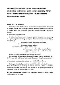
Hicksian vs. Marshallian Demand
Hicksian Demand x2
p1
p1
p1 Hicksian demand curves are steeper for normal goods
Hicksian demand curves are flatter for inferior goods
Decreasing p1 DHicksian
DMarshallian DHicksian x1 Spring 2001
x1
Econ 11--Lecture 7
7
Spring 2001
8
Law of Demand • Hicksian Demand Curves must slope down.
• Recall Slutsky Equation
Compensated
x1
Econ 11--Lecture 7
Hicksian Demand Functions dx1 dx = dp1 dp1
DMarshallian x1
– Why? The substitution effect is negative.
dx − 1 x10 dI
x2
• Hicksian (or Compensated or Utility constant demand functions) yield the amount of good x1 purchased at prices p1 and p2 when income is just high enough to get utility level u0.
(
x1 = h p1 , p 2 , u 0 Spring 2001
)
x1
Econ 11--Lecture 7
9
Spring 2001
Econ 11--Lecture 7
10
Calculating Hicksian Demand
Calculating Hicksian Demand (II)
• For Hicksian demand, utility is held constant. • The trick to calculating Hicksian demand is to use expenditure minimization subject to a constant level of utility, rather than utility maximization subject to a constant level of income. • Expenditure minimization is known as the “dual” problem to utility maximization.
• Suppose U0=U(x1, x2) is a utility function at a given utility level U0 • Prices are p1 and p2. • Total expenditures are p1x1 + p2x2 • The expenditure minimization problem is:
Spring 2001
Spring 2001
min p x + p x 2 2 x1 , x2 1 1
s.t. U ( x1 , x2 ) = U 0
Econ 11--Lecture 7
Econ 11--Lecture 7
11
Econ 11--Lecture 7
12
2
Professor Jay Bhattacharya
Spring 2001
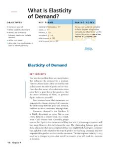
Net Complements and Net Substitutes
Calculating Hicksian Demand (III)
• Assume 3 goods, x1, x2, and x3 • Define x1 and x2 as “net substitutes” if an increase in the price of good 2 leads to an increase in the compensated demand for good 1.
• We can set up the Lagrangian objective: max L = p x + p x − λ (U ( x , x ) − U ) 1 1 2 2 1 2 0 x1 , x2
• The solution to this problem will be two Hicksian demand functions:
dx1 dp2
x1 = h1 ( p1 , p2 ,U 0 ) *
> 0 ⇒ net substitutes compensated
x2* = h2 ( p1 , p2 , U 0 ) Spring 2001
Econ 11--Lecture 7
13
Spring 2001
Econ 11--Lecture 7
Net Substitutes Increase in p2 Increase in x1 slope = −
Net Complements
Í
• Define x1 and x2 as “net complements” if an increase in the price of good 2 leads to an decrease in the compensated demand for good 1.