iBusiness, 2010, 2, 218-222 doi:10.4236/ib.2010.23027 Published Online September 2010 (http://www.SciRP.org/journal/ib)
DCC and Analysis of the Exchange Rate and the Stock Market Returns’ Volatility: An Evidence Study of Thailand Country Wann-Jyi Horng, Ching-Huei Chen Department of Hospital and Health Care Administration, Chia Nan University of Pharmacy & Science, Tainan, China. Email:
[email protected],
[email protected] Received June 4th, 2010; revised July 9th, 2010; accepted August 10th, 2010.
ABSTRACT This paper studies the relatedness and the model construction of exchange rate volatility and the Thailand’s stock market returns. Empirical results show that we can construct a bivariate IGARCH (1, 1) model with a dynamic conditional correlation (DCC) to analyze the relationship of exchange rate volatility and Thailand’s stock market returns. The average estimation value of the DCC coefficient for these two markets equals to –0.1650, this result indicates that the exchange rate volatility negatively affects the Thailand’s stock market. Empirical result also shows that there do not exist the asymmetrical effect on the Thailand’s exchange rate and Thailand’s stock markets. And the Japan’s stock return volatility truly affects the variation risks of the Thailand stock market. Based on the viewpoint of DCC, the bivariate IGARCH (1, 1) model with a DCC has the better explanation ability compared to the traditional bivariate GARCH (1, 1) model. Keywords: Four Quadrant (4Q) Converter, Interlacing, Traction Systems, Power Quality Analysis
1. Introduction We know that Thailand belongs to the Buddhism country. And Thailand is also a famous scenic spot of travel. Besides, Thailand is also one of Association of South-east Asian Nations in the global economical financial system and also has been very influential in the global economy. We also know that the relationships between stock prices and foreign exchange rates are studied of numerous economists, because they both play crucial roles in influencing the development of a country’s economy. A study of the exchange rates affects the stock returns, for example, Kearney [1] found that the exchange rate volatilities in Canada and Ireland had a significance influence on their stock market volatilities. Besides, we also can refer to, for example, the papers of Bollerslev [2], Nieh and Lee [3], and Yang and Doong [4]. Therefore, the relationships of the foreign exchange rates and the stock market will also become an important topic. In this paper, we will consider the factors of the foreign exchange rates to discuss it on the stock market’s influence. An evidence study of the Thailand’s stock market is considered. We also know that Japan is one of eight big industrialized
Copyright © 2010 SciRes.
countries in the global economical financial system. In the year 2006, for example, the turnover of the Japan’s Tokyo stock market achieves to US5,497 billion, which is only inferior to the New York and London stock exchanges. Therefore, we are also considered the influence factor of Japan’s stock market in Thailand. In this paper, the Student’s t distribution is adopted and the maximum likelihood algorithm method of BHHH [5] is used to estimate the model’s unknown parameters. The programs of RATS and EVIEWS are used in this paper. This paper is organized as follows. Section 2 states the data characteristics. Section 3 presents the asymmetric test of the bivariate GARCH model. Section 4 introduces the proposed models of DCC and GARCH. Section 5 presents the empirical results, and ends with Section 6 of conclusions.
2. Data Characteristics 2.1. Basic Statistics and Trend Charts In the sample selection, this research uses the Thailand stock index ( THAILt ), NK-225 stock index ( JAPANLt ) and the closed price of the Thailand’s exchange rate ( THERt )
iB
DCC and Analysis of the Exchange Rate and the Stock Market Returns’ Volatility: An Evidence Study of Thailand Country
of the Thailand dollars to the US dollars. The daily-based sample period is from January, 2000, to August 14, 2008, and the research data are collected from the Taiwan Economic Journal (TEJ), a database in Taiwan. The researcher adopts the natural logarithm with a step difference of 100 times to compute the return rate for the Thailand’s stock index-namely RTHAILt 100 * ln (THAILt / THAILt 1 ).
The Japan’s stock price return rate equals to RJAPANt 100* ln ( JAPANt / JAPANt 1 ).
The exchange rate volatility rate equals to RTHERt 100* ln ( THERt / THERt 1 ).
In Figure 1, the Thailand’s stock price return volatility, exchange rate return volatility, and the Japan’s. stock return volatility shows the clustering phenomenon, so that we may know the stock market and exchange rate market have certain relevance. By the unit root test as below, the Thailand’s stock index return rate, the Japan’s stock index return rate and the volatility rate of the exchange rate are all stationary sequences. The basic statisRTHAIL 15 10
219
tics of these sequences are stated in Table 1. According to Table 1, as shown by the Jarque-Bera statistics under the null hypotheses of normal distribution, these two markets do not obey the assumption of normal distribution. Therefore, the heavy tails distribution is used to evaluate the proposed mode l.
2.2. Unit Root Test and Co-Integration Test This paper further uses the unit root tests of ADF [6] and KSS [7] to determine the stability of the time series data. The ADF and KSS examination results is listed in Table 2. It shows that the Thailand’s stock index return, the Japan’s stock index return and the exchange rate return do not have the unit root characteristic−namely, the three markets are stationary time series data, under 1% significance level. By the cointegration test of Johansen [8], we know that the statistics of max is not significant under the level 5% in Table 3. This demonstrates that these three markets of the Thailand’s stock index, the Japan’s stock index and exchange rates do not have co-integration of their relations. Therefore, we are not considered the model of error correction.
5
Table 1. Basic statistics of the research data.
0
Statistics
-5 -10
Mean
-15
Standard deviation
-20 250
500
750
1000
1250
1500
1750
RTHER
J-B (p-value) Sample
8
RTHAIL
RTHER
RJAPAN
0.0178
−0.0046
−0.0196
1.5366
0.6068
11747.17 (0.000)
1.4642
143066 *** (0.000)
1768
1768
305.0880 (0.000) 1768
Notes: (1) J-B denotes the normal distribution test of Jarque-Bera. (2) *** denotes significance at level = 1%.
4
Table 2. Unit root test of adf and kss methods.
0
ADF
-4
RTHAIL
Statistic -8 250
500
750
1000
1250
1500
1750
Critical value KSS Statistic
RJAPAN 8
Critical value
RTHER ***
RJAPAN ***
−10.3556 44.8710 *** −42.3730 −3.963 ( = 1%), −3.412 ( = 5%) RTHAIL RTHER RJAPAN −18.4679 *** −33.6306 *** 22.2000 *** −2.82 ( = 1%), −2.22 ( = 5%)
Notes: *** denotes significance at the 1% level.
4 0
Table 3. Johanson co-integration test (var lag = 3).
-4 -8 -12 250
500
750
1000
1250
1500
1750
Figure 1. Tend chart of Thailand’s stock price index return rate, the return rate of exchange rate, and the Japan’s stock return.
Copyright © 2010 SciRes.
Null H 0
max
Critical value
None
17.6491
25.8232
At most 1
8.6794
19.3870
At most 2
4.3717
12.5180
Notes: The lag of VAR is selected by the AIC rule [9]. The critical value is given under the 5% level.
iB
220
DCC and Analysis of the Exchange Rate and the Stock Market Returns’ Volatility: An Evidence Study of Thailand Country
2.3. ARCH Effect Test Based on the Formulas (1) and (2) as below, we uses the methods of LM test [10] and F test [11] to test the conditionally heteroskedasticity phenomenon. In Table 4, the results of the ARCH effect test show that these two markets have the conditionally heteroskedasticity phenomenon exists. This result suggests that we can use the GARCH model to match and analyze it. The detail is omitted here.
4. Proposed Model A dynamic conditional correlation (DCC) and the bivariate GARCH (1, 1) model with an Japan’s. stock market factor is proposed in this section, its model may be expressed as
RTHAIL t 0 11 RTHER t 1
21 RTHAIL t 1 1 RJAPAN t 3 a1,t
(1)
Table 4. Arch effect test (lag = 15). Statistics (p-value) RTHER Statistics (p-value)
Engle LM test
Tsay F test
***
316.4800 (0.0000) Engle LM test
7.5925 *** (0.0000) Tsay F test
504.9780 *** (0.0000)
20.4977 *** (0.0000)
Notes: ** denotes significance at the level 5% and *** denotes significance at level = 1%.
Table 5. Asymmetric test of the bivariate igarch. RTHAIL
RTHER
Asymmetric test F statistic (p-value) Asymmetric test F statistic (p-value)
Positive size bias test 0.2893 (0.5907) Positive size bias test 0.5850 (0.4444)
Notes: p-value < denotes significance ( = 5%).
Copyright © 2010 SciRes.
h22,t = 20 + 21a22,t 1 21h22,t 1 + 2 a12,t 1
Joint test 0.4174 (0.7405) Joint test 0.6530 (0.5810)
(3)
(5)
qt 0 1 t 1 2 a1, t 1a2, t 1 / h11, t 1h22 , t 1 h12 , t t h11, t h22 , t
The bivariate IGARCH (1, 1) model with a DCC can be constructed in the next section. The asymmetric test methods [12] are used the following two methods as: negative size bias test and joint test. Table 5 asymmetrically examines the result for the Thailand’s stock market as: 1) The positive size bias test does not reveal ( = 10%). 2) The joint test does not reveal ( = 10%). Table 5 asymmetrically examines the result for the exchange rate market as: 1) The positive size bias test does not reveal ( = 10%). 2) The joint test does not reveal ( = 10%).
(2)
h11,t = 10 + 11a12,t 1 11h11,t 1 + 1 RJAPAN t21 (4)
t (exp (qt ) 1) / (exp (qt ) 1)
3. Asymmetric Test of the Bivariate IGARCH Model with a DCC
RTHAIL
RTHER t 0 11 RTHER t 1 21 RTHAIL t 1 2 RJAPAN t 3 a 2 ,t at' (a1,t , a2,t ) ~ Tv (0, ( 2) H t / )
(6) (7)
where Tv (0, (v 2) H t / v) denotes the bivariate Student’s t
distribution, its mean is equal to 0 and its covariance matrix is equal to (v 2) H t / v , and v is the degree of freedom. The DCC and the bivariate GARCH model can also refer to the papers of Engle [13] and Tse and Tsui [14].
5. Empirical Results From the asymmetric test results in Table 5, we can use the symmetric GARCH model to analyze the exchange rate and the Thailand’s stock markets. Table 6 shows the estimate results for the Thailand’s stock index return and exchange rate volatility rate by the DCC and the bivariate IGARCH (1, 1) model with a factor of Japan’s stock market. Empirical result shows that the Thailand’s stock market return receives the previous one period’s influence of the exchange rate volatility. Empirical result also indicates that the Thailand’s stock market return receives the previous one period’s influence of the Thailand’s stock return volatility. The Thailand’s stock market return also receives the previous third period’s influence of the Japan’s stock return volatility. Empirical result also shows that the exchange rate market return receives the previous one period’s influence of the exchange rate return volatility. Empirical result also indicates that the exchange rate market return receives the previous one period’s influence of the Thailand’s stock return volatility. The exchange rate market return does not receive the previous third period’s influence of the Japan’s. stock return volatility. Regarding the degrees of freedom of the Student’s distribution estimated value, it is 3.859, which under the 1% significance level is significant. Empirical result also shows that the variation risks of the exchange rate and the Thailand’s stock return volatility do have the different variation risks. Besides, the likelihood ratio test is also supported the proposed model under the Japan and non-Japan stock market factor. The details are omitted in this paper. And proposed model conforms to the parameters of the IGARCH and GARCH model’s supposition. From the above results, we can reiB
DCC and Analysis of the Exchange Rate and the Stock Market Returns’ Volatility: An Evidence Study of Thailand Country Table 6. Asymmetric test of the bivariate igarch. Parameter
0
11
21
Coefficient
0.0419
−0.0961
0.0599
(p-value)
(0.1054)
( 0.0302)
(0.0104)
Parameter
1
0
11
Coefficient (p-value)
0.0722
−0.0048
−0.0541
(0.0001)
(0.4632)
(0.0257)
Parameter
21
2
Coefficient
−0.094
−0.0006
(p-value)
(0.0000)
(0.8952)
Parameter
10
11
Coefficient (p-value)
11
0.1457
0.1839
0.7921
(0.0000)
(0.0000)
Parameter
1
20
21
Coefficient
0.0240
0.0187
0.3156
(p-value)
(0.0914)
(0.0000)
(0.0000)
Parameter
21
2
Coefficient
0.6467
0.00001
(p-value)
(0.0000)
(0.9870)
Parameter
0
1
−0.6615
−2.0047
0.0180
(p-value)
(0.0000)
(0.0045)
(0.2685)
t
−0.1650
3.8590
(p-value)
(0.0000)
(0.1914)
[1]
C. Kearney, “The Causes of Volatility in a Small, Internationally Integrated Stock Market: Ireland, July 1975 June 1994,” Journal of Financial Research, Vol. 21, No. 4, 1998, pp. 85-104.
[2]
T. Bollerslev, “Modeling the Coherence in Short-Run Nominal Exchange Rates: A Multivariate Generalized ARCH Model,” Review of Economics and Statistics, Vol. 72, No. 3, 1990, pp. 498-505.
[3]
C. C. Nieh and C. F. Lee, “Dynamic Relationship between Stock Prices and Exchange Rates for G-7 Countries,” The Quarterly of Economics and Finance, Vol. 41, No. 3, 2001, pp. 477-490.
[4]
S. Y. Yang and S. C. Doong, “Price and Volatility Spillovers between Stock Prices and Exchange Rates: Empirical Evidence from the G-7 Countries,” International Journal of Business and Economics, Vol. 3, No. 2, 2004, pp. 139-153.
[5]
E. K. Berndt, B. H. Hall, R. E. Hall and J. A. Hausman, “Estimation and Inference in Nonlinear Structural Models,” Annals of Economic and Social Measurement, Vol. 3, No. 4, 1974, pp. 653-665.
[6]
D. A. Dickey and W. A. Fuller, “Distribution of the Estimators for Autoregressive Time Series with a Unit Root,” Journal of the American Statistical Association, Vol. 74, No. 366, 1979, pp. 427-431.
[7]
G. Kapetanios, Y. Shin and A. Snell, “Testing for a Unit Root in the Nonlinear STAR Framework,” Journal of Econometrics, Vol. 112, No. 2, 2003, pp. 359-379.
[8]
S. Johansen, “Estimation and Hypothesis Testing of Cointegration Vector in Gaussian Vector Autoregressive Models,” Econometrica, Vol. 59, No. 6, 1991, pp. 1551-1580.
[9]
H. Akaike, “Information Theory and an Extension of the Maximum Likelihood Principle,” 2nd International Symposium on Information Theory, B. N. Petrov and F. C. Budapest, Eds., Akademiai Kiado, Budapest, 1973, pp. 267-281.
2
Coefficient Parameter
Thailand’s stock markets. The empirical results also show that the exchange rate volatility rate truly has an affect on the Thailand’s stock market return rate’s volatility. However, the proposed model is different from the traditional model of the bivariate GARCH. Based on the viewpoint of DCC, the DCC and the bivariate IGARCH model have a better explanatory ability compared to the traditional bivariate GARCH model.
REFERENCES
( 0.0001)
Coefficient
Notes: p-value < denotes significance ( = 1%, = 5%, = 10%);
is the significance level.
alize that the exchange rate and the Thailand’s stock market return’s volatility do not have an asymmetrical effect. The square item of the Japan’s stock return also affects the variation risk of the Thailand stock market. But the error square item of the Thailand’s stock return does not affect the variation risk of the exchange rate market. Therefore, the DCC and the bivariate IGARCH (1, 1) model with a Japan’s stock market factor might capture the exchange rate and the Thailand’s stock market return’s volatility process. To test the inappropriateness of the DCC and the bivariate IGARCH (1, 1) model with an U.S. stock market factor, the test method of Ljung & Box [15] is used to examine autocorrelation of the standard residual error. This model does not show an autocorrelation of the standard residual error, the details are omitted. Based on the paper of Engle [13], the DCC and the bivariate IGARCH (1, 1) model with a factor of Japan’s stock market are more appropriate.
6. Conclusions The empirical results present that the volatility process do not have an asymmetrical in the exchange rate and Copyright © 2010 SciRes.
221
[10] R. F. Engle, “Autoregressive Conditional Heteroskedasticity with Estimates of the Variance of United Kingdom Inflation,” Econometrica, Vol. 50, No. 4, 1982, pp. 9871007. [11] R. S. Tsay, “Analysis of Financial Time Series,” John Wiley & Sons, Inc., New York, 2004. [12] R. F. Engle and V. K. Ng, “Measuring and Testing the Impact of News on Volatility,” Journal of Finance, Vol. 48, No. 5, 1993, pp. 1749-1777. [13] R. F. Engle, “Dynamic Conditional Correlation - A SimiB
222
DCC and Analysis of the Exchange Rate and the Stock Market Returns’ Volatility: An Evidence Study of Thailand Country ple Class of Multivariate GARCH Models,” Journal of Business and Economic Statistics, Vol. 20, No. 3, 2002, pp. 339-350.
[14] Y. K. Tse and A. K. C. Tsui, “A Multivariate GARCH Model with Time-Varying Correlations,” Journal of
Copyright © 2010 SciRes.
Business & Economic Statistics, Vol. 20, No. 3, 2002, pp. 351-362. [15] G. M. Ljung and G. E. P. Box, “On a Measure of Lack of Fit in Time Series Models,” Biometrika, Vol. 65, No. 2, 1978, pp. 297-303.
iB