The 10th International Workshop on Wireless Network Measurements and Experimentation (WiNMeE 2014)
Crack STIT Tessellations for City Modeling and Impact of Terrain Topology on Wireless Propagation Xiaoxing Yu, Thomas Courtat, Philipe Martins, Laurent Decreusefond
Jean-Marc Kelif
Department of Information and Networks TELECOM ParisTech (ENST)
Orange Labs Issy-Les-Moulineaux, France
different cities according to their ξ and MBBA. Conclusions on wireless propagation for that specific deployments can then be drawn. This work proposes to model building deployments in cities by using crack STIT tessellations. It investigates the impact of crack STIT tessellations parameters on received power and path-loss exponent. The research carried out in this work relies on a two step methodology: a) generation of city according to a crack STIT tessellation model; b) use of 3D ray tracing algorithms to compute received power distributions in the generated city map. The rest of the paper is organized as follows. Section II introduces some theoretical background about crack STIT tessellations. Their generation process will be outlined. The anisotropy and the MBBA parameters will also be defined. Section IV investigates the practical impact of ξ and MBBA on path-loss exponent γ by simulations. It also studies the evolution of outdoor to overall area ratio (Free Area Ratio, FAR) versus ξ and MBBA. Finally some future directions of investigation and conclusions are drawn in section V.
Abstract—This work proposes to model city maps with a particular family of random tessellations: Crack STIT tessellations. This family of tessellations allow the generation of realistic city maps with a reduced number of parameters: the Anisotropy Ratio (ξ) and the Mean Building Block Area (MBBA). These city models are then used as input to a 3D ray tracing simulator to compute received power distributions. The objective of this investigation is to identify the impact of random tessellation parameters on wireless propagation. For this purpose, path loss exponent γ is estimated from received power distributions obtained by simulation for different values of ξ and MBBA pairs. Simulations results clearly show a linear dependency between path loss γ, ξ and MBBA. Path loss γ increases with ξ while it decreases with MBBA. Furthermore the evolution of the surface occupation ratio between outdoor and overall surface is also investigated. This ratio is named Free Area Ratio (FAR) in the sequel. It decreases with MBBA according to a power law. The results obtained are particularly promising as they provide a parametric relation between path loss exponent γ and terrain topology. This considerably simplifies the radio planning and dimensionning process of cellular networks. Index Terms—random tessellations, crack STIT, anisotropy ratio, mean building block area, propagation impact, path loss exponent
II. C RACK STIT T ESSELLATIONS BACKGROUND I. I NTRODUCTION
A. Preliminaries
The development of modern wireless communication technologies, such as LTE and LTE advanced, will require the use of more tractable and accurate propagation models. More realistic estimations of the received power and of the interference levels will be needed for a better capacity estimation and planning. One of the major issues in propagation modeling is the design of a model that integrates the impact of the terrain topology in wireless propagation. Many statistical propagation models already exist in the literature but they are obtained from experimental measurements and cannot be transposed to different urban environments. Stochastic geometry can be a valuable tool in modeling terrain topology in a urban context. Some families of random tessellations, namely crack STIT tessellations, can be used to model and generate realistic city maps and building deployments. They concentrate topology description of terrain in a small set of parameters: Anisotropy Ratio (ξ) and Mean Building Block Area (MBBA). They are also quite easy to simulate. These features makes them particularly attractive for investigating the effects of terrain topology on wireless propagation channel. As a matter of fact it is possible to classify
978-3-901882-63-0/2014 - Copyright is with IFIP
Let L be a line in the Euclidean plane with origin oL and direction vector uL . It divides R2 into two disjoint regions: L+ = {x ∈ R2 , det(ul , (x − ol )) > 0} and L− = {x ∈ R2 , det(ul , (x − ol )) < 0}. The set of lines in the plane is written H and the set of polygons possibly infinite is P. In the following we consider the function: D: P×H → P×P (1) (P, L) → (P ∩ L+ , P ∩ L− ) This function can beSextended to a set of convex polygons: {Pi }: D({Pi }, L) = i {Pi ∩ L+ , Pi ∩ L− }. It separates one set of polygons crossed by one random line into two smaller sets of polygon-es. B. General definitions Definition 1: A tessellation Ξ is a countable family of convex polygons {Ci }i∈N (the cells) whose interiors do not intersect. The dual definition can also be adopted: a tessellation is a straight planar graph whose vertexes are the cells’ vertexes and
22
The 10th International Workshop on Wireless Network Measurements and Experimentation (WiNMeE 2014)
edges are cell’s. When considered as a family of polygons, the tessellation writes Ξ and when considered as a graph ∂Ξ. To handle randomness with tessellation, the set of tessellations is equipped with the σ-algebra generated by sets {Ξ, ∂Ξ ∩ K = ∅} where K is a compact part of R2 [1]. Generally, a tessellation P is deducted from a point process. For instance, if X = Xi is a Poisson Point Process in the plane and if to each point Xi is associated its Vorono¨ı zone V (Xi ||X), {V (Xi ||X)}i is then a random tessellation named Poisson Vorono¨ı Tessellation [2].
D. Construction Random Line and Poisson Line Tessellation: We start by describing the construction of a Poisson Line Process. To a line L is associated πd (o), the projection of the plane’s origin o onto this line. The signed distance between the line L and the origin is define by ||πd (o) − o||.sgn(hπd (o) − o | t(1 , 0)i). Definition 2: The Poisson Line Process (PL) ∂Ξ of intensity measure λ and anisotropy measure R is the Poisson Point Process on the cylinder R × [0, π[ of intensity L(.) = λµ(.) ⊗ R(.), λ > 0. The associated Poisson Line Tessellation (PLT) Ξ is the random set of the connected components of R2 \∂Ξ. These two processes (generically written Ξ in what follows) have two fundamental properties: Property 1: Ξ is stationary: if . + ~v is the translation of dist vector ~v then Ξ = Ξ + ~v . The statistical properties of a PL or a PLT are the same wherever they are observed. Property 2: Ξ is locally finite: if W is a compact of R2 then L(H ∩ W ) = L({h ∈ H, h ∩ W 6= ∅}) < ∞. Consequently to simulate the intersection of an infinite PLT with a compact window W : Ξ ∩ W , Ξ ∼ L, is the same as to simulate the intersection of W with the finite process of intensity LW (.) = L(. ∩ W ). Property 3: If C is a circle with radius r then ]LC (.) follows a Poisson Law of parameter λ.2.r whatever R is and conditionally to it cuts C, a line of the process has a distance to the center of C uniformly distributed. Furthermore, if W ⊂ C then LW (.) = LW ∩C (.) = LC (. ∩ W ). It is sufficient to draw a Poisson Line in C and keep only lines that cross W which leads to the simple algorithm 1 to simulate the intersection of a PLT with W .
C. Model choice Many random tessellation models have been proposed to represent street systems in the cities. For instance, [3], [4] suggests to use Poisson Vorono¨ı. [1], [2], [5] and [6] propose models based on Poisson Line Tessellation and Crack STIT Tessellation. More recently, it has been shown in [7], [8] that a city’s morphology can result from two growth mechanisms. The first one is an organic like growth: independent agents divide sequentially plots of land to settle in. Agents do not consult each other, consequently axis they create are not coherent and street intersections are T-shaped. Conversely in the case of a planned deployment of cities, agents act under an authority and draw long transportation axis to optimize displacements within the city. Crack STIT tessellations can mimic these different situations (Fig.1). These two models are quite similar and can be treated in the same theoretical framework. Indeed they both result from sequential divisions of polygons and if edges in a Crack STIT were extended into infinite line, one would obtain a Poisson Line Tessellation. This has for consequence that the typical cell of the tessellations are equal in distribution [9]. They both depend on two parameters: an intensity parameter λ ∈ R+ and a probability measure R that describes the anisotropy of the street system [9].
Algorithm 1 Ξ = PLT(λ, W ) Poisson Line Tessellation process intersected by W 1: 2: 3: 4: 5: 6: 7: 8: 9: 10: 11: 12: 13: 14: 15: 16:
Fig. 1: Realization of tessellations into a disc. The first row shows PLT with from left to right an anisotropy of 0, 0.5 and 1. The second row shows Crack STIT with the same anisotropy distributions.
INPUT λ ∈ R+ , W OUTPUT: Tessellation Ξ Tessellation T0 = {W } Inscribe W in a circle C of center 00 and radius r. N ∼ P(λ.2r) ; n = 1 while n ≤ N do r0 ∼ U[−r,r] ; α ∼ R Consider the line l = (r0 , α) + 00 if d ∩ W 6= ∅ then Ξn = D(Ξ, l) n++ else Ξn = Ξn−1 end if end while Ξ = ΞN
The choice of the smallest circle circumscribed to W permits to minimize line rejections and thus to improve running time.
23
The 10th International Workshop on Wireless Network Measurements and Experimentation (WiNMeE 2014)
Algorithm 2 l ∼ LW Random line in W 1: 2: 3: 4: 5: 6: 7: 8: 9:
(these formulae remain true for all Borelian of area 1 if the tessellation is isotropic i.e. if R is uniform or if ρ = 2/π). Knowing these mean formulae permits to calibrate the models to fit real data.
INPUT W Inscribe W in a circle of center 00 and radius r.. while do r0 ∼ U[−r,r] ; α ∼ R Consider the line l = (r0 , α) + 00 if d ∩ W 6= ∅ then return l BREAK end if end while
Crack STIT: A Crack is a division of space process. Unlike PLT, it is defined sequentially in a bounded window and [6] shows that this bounded process can be extended to a random tessellation in the whole plane. Informally, at a time t, the tessellation is Ξt = {Ci } and dt, each cell Ci in the tessellation has a probability λ.ν(Ci ).dt, λ > 0 to be divided into two new cells and a probability o(dt2 ) to be divided twice. ν(.) is a positive measure on the set of convex bodies, invariant under rigid motion (for instance area, perimeter, number of vertexes) [10]. The tessellation is observed at a finite time τ , the homogeneous quantity λ.τ describes the intensity of the process in such a way one can come down to τ = 1. If the measure ν is the perimeter (which is the case under consideration in what follows), the resulting tessellation process has interesting properties: it is STable under ITeration (STIT) and its typical cell is equal in distribution to the PLT’s one. Algorithmic-ally the Crack’s construction can be made recursively with the function division D and a generator of the law Lω with ω a compact set. To do this, we define the auxiliary function of evolution of a cell C belonging to a tessellation Ξ from a time t > 0:
Parameters
Notation
Total edge length Number of vertices Number of edges Number of cells Length of the typical edge Perimeter of the typical cell Area of the typical cell
LA N0 N1 N2 U1 U2 A2
Mean value per u.a for PLT λ 1 ρλ2 2 λ2 ρ 1 2 λ ρ 2 2/(3λρ) 4/(λρ) 2/(λ2 ρ)
Mean value per u.a for Crack λ.τ L2A ρ 3 2 L ρ 2 A 1 2 L ρ 2 A 2/(3LA ρ) 4/(LA ρ) 2/(L2A ρ)
TABLE I: Expectancies of various morphological features of PLT and Crack STIT in function of their intensity λ and their anisotropy parameter ρ. In a city modelling context, the particular family of angular distribution Rξ , ξ ∈ [0, 1] is under consideration with: ξ Rξ = (1 − ξ)U[0,π] + (δθ + δθ+π/2 ) (3) 2 Where θ is a constant tessellation initial direction vector. Samples can be generated easily from Rξ and this family allows to go continuously from an isotropic network (ξ = 0) to an anisotropic Manhattan-like one (ξ = 1). For this family of distributions, ρ writes: 2 2 1 ρ(ξ) = ξ 2 ( − ) + 2 π π III. B UILDINGS GENERATION
(4)
The tessellation represent the street axis (alignments of edges), the city skeleton (Fig.2,1). From this, axis are thickened with a Minkowski’s sum ⊕� , � > 0. If A is a subset of the plane, ⊕� A = {x ∈ R2 , d(x, A) ≤ �} (5)
Algorithm 3 evolution(C, t, Ξ, τ, λ) δt ∼ E(λ.ν(C) if t + δt < τ then L ∼ RC , (C+ , C− ) = D(C, L) Ξ = (Ξ − {C}) ∪ {C+ , C− } 5: evolution(C+ , t + δt, Ξ, τ, λ) 6: evolution(C, t + δt, Ξ, τ, λ) 7: end if 1: 2: 3: 4:
Property 4: If {Ai } are the axis of a tessellation, i.e subsets of edges that are aligned, the connected components of R2 \ ⊕� ∪ Ai , � > 0 are polygons Bi that do not intersect. If {Ci } is the set of cells of the tessellation then each Bi is the image of a cell Ck by the operator � �/2 (C) = {x ∈ C, d(x, ∂C) > } (6) 2 We can thus shape building blocks (Fig.2,2) by applying �/2 independently to each cell in T . Computational, �/2 C is equivalent to the sequential division of C by its edges shifted of a distance �/2 toward its interior. Once blocks obtained, we associate to each block B its image by the dilatation of center its center of mass and ratio ˜ (Fig.2,3). η: B A Poisson Point Process of intensity 1/(b.η) is drawn on the ˜ ˜b1 , ..., ˜bN , ˜bN +1 = ˜b1 , these points external frontier of B, ∂ B: being sorted clockwise (Fig.2,4). We write bi the projection of ˜bi on ∂B (internal frontier of B) and qi,1 , qi,2 ..qi,ni the vertices of ∂B sorted clockwise from bi to bi+1 .
Definition 3: There exist a stationary, locally finite tessellation whose intersection with a convex and compact window W is the result of crack(W, τ, λ) = evolution(W, 0|{W }, τ, λ). It is called the Crack STIT tessellation. E. Mean formulae Mean formulae (Tab.I, [9]) are known for topological features of PLT and Crack STIT in a disc of area 1 in function of their intensity λ and of the so called anisotropy parameter: ZZ def | sin ](u, v)|R(du)R(dv) (2) ρ=
24
The 10th International Workshop on Wireless Network Measurements and Experimentation (WiNMeE 2014)
We then create polygons ˜bi , pi , qi,1 , qi,2 ..qi,ni , bi+1 , ˜bi+1 , ˜bi to represent buildings’ footprints (Fig.2,5). Finally, to each building is associated a random height from a distribution E(h), h > 0. From now, we can generate buildings whose mean fac¸ade length and mean height are known: b and h. Figure 3 shows two city maps obtained by applying the previous computational steps.
IV. T ERRAIN T OPOLOGY I MPACT M ECHANISM A SSUMPTION From the above introduction, we can clearly find out that Anisotropy Ratio ξ (also called AR) basically controls the tessellation of the city, which includes the direction of the streets and the shape of divisions and building blocks. In a sense, it also determines the potential propagation channel orientations. MBBA is the average area of a block. It controls the size of the obstacles directly, which would further influence the “free space/occupation”ratio and the length of the walls that forming the propagation channels as it is illustrated in in Fig.3. A. Key Propagation Term Based on this power map, two variables are selected as the evaluation criteria related to the propagation. One is the Free Area Ratio (FAR), the other one is the general path-loss exponent γ. FAR is the ratio between the area of all free grids which have receiving values (denoted as Af i ) and all scanned grids area (denoted as AH ). FAR can tell us the vacancy of the region, and the outdoor user mobiles can only be assumed to deploy in these free receiving regions. It is a highly user related criteria that we will go further researches in future works. Meanwhile, γ is derived from the spatial relationship itself. It is also a key parameter of evaluating the wireless service. In our assumption, FAR is clearly affected by environmental parameters like AR and MBBA, so it can be expressed as follow in Eq.7:
Fig. 2: Steps in the building generation. From a tessellation (1) we apply an erosion operator to axis (2) in each new cell, we compute its dilated polygon with respect to its center of mass (3) we draw on this polygon a Poisson Point Process (4) whose points are projected to create buildings’ footprint (5)
P F AR =
(a) ξ = 0.1, MBBA= 10000m2
i Af i (%) = f (M BBA, AR, . . .) , AH � f (M BBA) orF AR ∼ g (AR)
The general path-loss exponent γ is also calculated for each map. It can reveal the difficulty of the overall propagation process under certain environmental settings. It is estimated from the relation of obtained receiving power Pri and direct transmitter-receiver Euclidean distance Di in Eq.8. It is also assumed to be related to MBBA and AR like Eq.9 shows. Smaller γ means slower attenuation and easier propagation and better signal intensity and service.
(b) ξ = 0.9, MBBA= 10000m2
Pri =
G×C Diγ
γ = f (M BBA, AR, . . .)
(c) ξ = 0.5, MBBA= 2500m2
(7)
(8)
(9)
Where G is the constant of antenna gain, and C is the constant part including frequency. 1) Impact Mechanism Assumption: In the generation process using Crack Tessellation, MBBA will directly influence FAR via controlling the block size, while the main factor brought by AR is the map randomness. Smaller AR brings bigger randomness. And randomness can affect the building Generation Step (GS) of Crack Tessellation termination and
(d) ξ = 0.5, MBBA= 40000m2
Fig. 3: Map examples: White for buildings and red for outdoor region
25
The 10th International Workshop on Wireless Network Measurements and Experimentation (WiNMeE 2014)
Where di is the propagation distance between each two reflections, and each reflection brings a reflection attenuation coefficient AT Ti . C 0 and C 00 are the sum of the transformed constant parts. Thus, for reaching a fixed mobile position, shorter di with more reflection number M results to smaller Pri because of more frequent reflections. And these accumulated attenuations AT Ti will decrease Pri rapidly. Meanwhile, Di of this mobile is fixed for different city structures and propagation. Thus, combining the right side of both Eq.10 and Eq.11, we can conclude that the fast fading away power will make the observing γ seem to be bigger according to Eq.12. X γ ∝ log d2i + M log AT Ti + C 000 (12)
building Coverage Efficiency of Grids (CEG) which means the easiness and efficiency of how many building blocks can cover a grid. Combining the grid size, AR may affect FAR in the following ways: • Smaller AR means more messy trivial shape of building blocks and space occupation, while big AR means neater and more unified space utilization. The irregularity of the block shape can interference and waste some neighbor free grids, and may bring “fake” high CEG, like Fig.4 shows. • AR may also affect GS according to specific MBBA requirement. If MBBA is large enough, the random convex may fulfill “big area” division easier than rectangles, and bring less blocks and more inner free space (like stadium), since the center of blocks may also be free according to logical design of building thickness. The simple illustration is shown in Fig.5.
M 000
Where C is the transformed general constant part. Back to each reflection, we believe that di and M is influenced by the randomness brought by ξ and Continuous Wall (CW) length of building block mainly brought by MBBA. Longer CW and bigger randomness bring less (bigger M ) and longer di due to less frequent short reflections. So, the assumption about γ is the following: • For MBBA, although bigger building seems to be more space assuming, bigger MBBA will bring longer CW which can ensure better continuous space for less and longer di to destiny. The propagation within the compressed space could be better guided channels (smaller M and longer di ) rather than frequent free reflections on small trivial building blocks, like in Fig.6. So the general γ in these canyons could be smaller. • For AR, smaller AR means more randomness. Compared with more unified rectangular tessellation, random division may generate more “corner plaza” with more flexible reflection angles. More rigid monotonous 90◦ block corners may be harder for a radial propagated nonzero incident signal, and thus brings shorter di , bigger M and bigger γ. It can also be called as “corner hardness”, like in Fig.7.
Fig. 4: Two more neighbor grids (G2 and G3) are interferced to be occupied due to smaller ξ for small MBBA
Fig. 5: More GS and blocks by bigger ξ when MBBA is big, which squeeze the free space For analyzing γ, it is better to study the propagation process in detail. Firstly, Eq.8 can transform into logarithm mode: � � G×C log Pri = log = C 0 + [(−γ) log Di ] (10) Diγ
(a) furthest distance is red after 3 (b) furthest distance is blue after reflections at the road end 3 reflections at the road end
Fig. 6: Longer CW ensures longer guided canyon, longer maximal radial propagation distance and faster to destiny with less reflections: red lines are the same radial lengths
The receiving power can also be expressed hop by hop when considering M reflection steps: " # X 2 00 log Pri = C + (−1) log di + (−M ) log AT Ti (11)
V. S IMULATION AND A NALYSIS The simulations will compute the receive power in outdoor regions of generated city maps using a 3D ray tracing simu-
M
26
The 10th International Workshop on Wireless Network Measurements and Experimentation (WiNMeE 2014)
FAR roughly before 10000 m2 MBBA. When MBBA grows larger, this phenomenon becomes more blur. 100
Area Ratio (%)
Anisotropy Ratio 0.1
(a) 4 reflections to destiny (b) 2 reflections to destiny with ranwith rigid corner degree dom corner degree
90
Anisotropy Ratio 0.3
80
Anisotropy Ratio 0.5 Anisotropy Ratio 0.7
70 Anisotropy Ratio 0.9 60 50 40
Fig. 7: Bigger ξ and rigid corner brings more reflections to destiny: red lines are the same radial lengths
30 0
2
4 6 Mean Building Block Area in m2
8
10 4 x 10
Fig. 8: FAR vs MBBA curves for different fixed ξ lator. The area of study will be a circular region with 1 km radius. The received power will be computed in the horizontal plane corresponding to an elevation of 1.5 m. The street width is fixed to 20 m, and the building height is fixed to 25 m. Antenna is set to the top of the closest building with extra 6 m tower height. The leaning angle of the antenna is 40◦ with ±40◦ scanning range, while the rays resolution is set to 107 beams. The transmitter has 40 W transmission power and 0.15 m wavelength (for 2 GHz frequency) with a fixed 50% reflection absorption coefficient. The background noise power is set to 10−12 W . A single ray will experience at most 100 reflections to stop. The simulator will compute the receiving power values for the entire region. Then the data will be sorted by grids according to the 2D radial distance to the antenna position “ring” by “ring”. The grid can be rectangular as well, but the radial grid has been selected for identifying the relation between the radial distance and the pathloss exponent γ. Considering the acceptable coverage estimation and effective power, we only count the receiving power of area within 300 m radius. In the following groups of simulations, the anisotropy ξ is scaled to 0.1, 0.3, 0.5, 0.7 and 0.9, while MBBA is scaled in square root from 25 m to 300 m with 25 m interval, which is from 625 m2 to 90000 m2 . More than 10000 power maps are generated for each ξ-MBBA . The curve fitting results provide the coefficients fitting and the Sum Standard Error (SSE) as well.
Fig.9 reveals the ξ-FAR relation and supports our above assumptions about it. When MBBA is small at first, smaller ξ brings bigger randomness, and FAR is increasing with bigger anisotropy. Compared with 20 m street width, small ξ with small MBBA brings huge randomness and division irregularity, which makes the fake high CEG dominates the FAR changing. Then, for moderate MBBA, the larger block size and less GS weaken the fake CEG effect of randomness until it reaches a balance like the “V” shape in a small range. Finally, when MBBA is very big, less GS brings less blocks and more free inner space due to small values of anisotropy. The block size surpasses the grid size, and makes rigid division establishing high CEG, and thus, big rectangles are overcovering. FAR turns to decrease with bigger ξ. 48
80
Free Area Ratio (FAR %)
Free Area Ratio (FAR %)
82 2
MBBA 2500m
78 76 74 72
0.1
0.3 0.5 0.7 Anisotropy Ratio (ξ)
In this section, the FAR evolution is studied along with the changing of ξ and MBBA. The same data are sorted into two types of curves. One is group of curves with fixed ξ, and the other one group with fixed MBBA. From Fig.8, we can see that the MBBA can strongly affect FAR. As MBBA grows larger from 625 m2 to 90000 m2 , FAR is monotonically decreasing, which leads to less free propagation space and user deployment space. It is clear that bigger building blocks will bring less free space. Meanwhile, Fig.8 also implies that ξ can slightly affect FAR at certain circumstances. The curves show that bigger ξ will bring bigger
44 0.3 0.5 0.7 Anisotropy Ratio (ξ)
0.9
40 MBBA 50625m2
41.5 41 40.5 40
45
0.1
Free Area Ratio (FAR %)
Free Area Ratio (FAR %)
A. Impact on Free Area Ratio
MBBA 30625m2
46
0.9
42.5 42
47
0.1
0.3 0.5 0.7 Anisotropy Ratio (ξ)
0.9
MBBA 90000m2
39.5 39 38.5 38 37.5 37 36.5
0.1
0.3 0.5 0.7 Anisotropy Ratio (ξ)
0.9
Fig. 9: FAR vs ξ curves for different MBBA Since the ξ-FAR relation has multiple patterns and changes gradually, no easy fitting has been selected to fit all the
27
The 10th International Workshop on Wireless Network Measurements and Experimentation (WiNMeE 2014)
TABLE II: MBBA-FAR power law fitting a
b
c
SSE
0.1 0.3 0.5 0.7 0.9
3.223 3.003 2.81 2.943 6.547
-0.2109 -0.1808 -0.1313 -0.08922 -0.02303
0.09088 -0.0126 -0.2719 -0.7057 -4.677
0.001613 0.001576 0.001466 0.001729 0.001249
MBBA 5625m2
patterns. However, the Power Law fits well the MBBA-FAR data in Fig.8. It means that the FAR can be fitted with a power law with MBBA like in Eq.13 with specific coefficient fitting results in Table.II. F AR = a × M BBAb + c + o [g (ξ)]
MBBA 75625m2
3.6
3.4
3.2
3
0.3
0.5
0.7
0.9
Fig. 11: General γ vs ξ curves for different MBBA TABLE III: MBBA-γ linear fitting
(13)
0.1 0.3 0.5 0.7 0.9 ξ 0.1 0.3 0.5 0.7 0.9
2500m2 ∼ 90000m2 p(10−6 ) q sse -9.637 -9.695 -9.582 -9.879 -10.99
3.464 3.49 3.52 3.587 3.687
0.04711 0.04297 0.04516 0.04707 0.05051
2500m2 ∼ 50625m2 p(10−6 ) q sse -12.43 -12.35 -11.86 -12.83 -13.79
3.515 3.54 3.563 3.639 3.739
0.02419 0.02028 0.02792 0.02295 0.02579
2500m2 ∼ 40000m2 p(10−6 ) q sse -13.7 -13.31 -13.25 -14.17 -15.05
3.532 3.553 3.581 3.656 3.755
0.02019 0.01798 0.02311 0.01847 0.02184
5625m2 ∼ 50625m2 p(10−6 ) q sse -10.71 -10.76 -10.03 -11.18 -12.13
3.455 3.484 3.498 3.581 3.681
0.00216 0.001516 0.002961 0.002679 0.005378
The simple linear fitting seems enough to describe the overall evolution of γ with MBBA and ξ, especially for the common moderate block size part from 2500m2 to 50000 m2 . Thus, it possible to convert the relation in previous Eq.9 into Eq.14: � p × M BBA + q γ∼ ,γ ≥ 2 (14) p0 × M BBA + q 0
4 Anisotropy Ratio 0.1 General pathloss exponent γ
MBBA 50625m2
Anisotropy Ratio
In this section, the general evolution of path loss exponent γ is studied along with the changing of ξ and MBBA. γ is the average of more than 10000 maps for each ξ-MBBA pair. The same data are also sorted with fixed ξ and fixed MBBA. Fig.10 and 11 shows the general γ sorted by increasing MBBA and increasing ξ separately. Despite the 625m2 data (labeled 25 in Fig.10 and decreasing curve in Fig.11), γ is monotonically decreasing with increasing MBBA. Bigger ξ will mostly bring slightly bigger γ. These results support our guided channel assumptions about MBBA-γ relation and rayentrance variety versus corner hardness assumptions about ξ-γ relation.
Anisotropy Ratio 0.3 Anisotropy Ratio 0.5 Anisotropy Ratio 0.7 Anisotropy Ratio 0.9
3.4
2
MBBA 30625m
0.1
B. Impact on Path-loss Exponent
3.6
MBBA 15625m2
2.8
ξ
3.8
MBBA 625m2
3.8
general pathloss exponent γ
ξ
4
3.2 3
The coefficient fitting results for Eq.14 are listed below in Table.III and IV. Table.III is divided into different MBBA fitting ranges to find most linear-like segment. Table.IV is consistent except for the 625 m2 data in the first row. Since both ξ and MBBA shows a linear relation with γ, the joint relation function in Eq.9 can also be concluded as a single plane function in Eq.15 by merging these two linear relations. The joint γ-MBBA-ξ surface is shown in Fig.12. Again, for more common moderate building block size from 2500m2 to 50000m2 , the surface is almost a flat plane. The whole surface can also be regarded as a piecewise plane with 3-4 linear stages like example shown in Fig.13. The following Table.V and VI list the coefficient fitting of Eq.15 for both single plane and piecewise plane.
2.8 2.6 0
2
4 6 Mean Building Block Area in m2
8
10 4 x 10
Fig. 10: General γ vs MBBA curves for different ξ The potential reason about the inconsistent data at 625 m2 is that the blockage size is too small when compared with 20 m street width. Rather than generating continuous reflections, the small blockages might be “invisibly bypassed”. These may result to the increase at 625 m2 in Fig.10. Moreover, for these small “gapping” obstacles, more rigid corner closer to 90◦ (bigger anisotropy) might be easier to proceed propagation in certain directions and encounter less reflections due to easier been bypassed. And this might be the reason of the decreasing dotted curve of 625 m2 in Fig.11.
γ = p1 × M BBA + p2 × ξ + q, γ ≥ 2
28
(15)
The 10th International Workshop on Wireless Network Measurements and Experimentation (WiNMeE 2014)
TABLE IV: ξ-γ linear fitting MBBA
3.7 3.6
Linear fitting result q0 sse
p0
625 2500 5625 10000 15625 22500 30625 40000 50625 62500 70625 90000
-0.5457 0.2664 0.2889 0.2528 0.24 0.2135 0.2255 0.2137 0.1984 0.2054 0.1454 0.1434
3.761 3.555 3.372 3.295 3.227 3.17 3.082 2.994 2.902 2.815 2.745 2.652
3.5 3.4
0.01405 0.002457 0.00334 0.002782 0.001123 0.0009285 0.0005435 0.0008599 0.0003695 0.004217 0.0007508 0.0001438
General γ
(m2 )
3.3 3.2 3.1 3 2.9 2.8
0 0.1 0.3 0.5 0.7 0.9 0.5
Anisotropy Ratio
1
1.5
2
2.5
3
3.5
MBBA in (m2)
4.5
4
5
4
x 10
Fig. 13: Piecewise fitting for MBBA 5625m2 ∼ 50625m2 in stage 3
TABLE V: ξ-MBBA-γ surface fitting (overall) MBBA 625m2
90000m2
∼ 2500m2 ∼ 90000m2
p1 (10−6 )
p2
q
sse
-9.773 -9.957
0.1540 0.2176
3.462 3.441
0.4915 0.2517
resource allocation performance (for example the number of resource blocks allocated in one area for a distribution of base stations and mobiles). We plan also to develop new methods that will help to infere anisotropy and MBBA for real cities maps or differant areas in a city. This will allow the identification of geoagraphical areas with common path loss exponent. Such classification will considerably ease the dimensionning and planning process of cellular networks.
TABLE VI: ξ-MBBA-γ surface fitting (4-stages) MBBA
p1 (10−6 )
p2
q
sse(10−3 )
625m2 ∼ 2500m2 2500m2 ∼ 10000m2 5625m2 ∼ 50625m2 50625m2 ∼ 90000m2
106.5 -34.69 -10.96 -7.101
-0.1396 0.2694 0.2333 0.1732
3.492 3.617 3.423 3.274
148.4 20.80 25.64 7.038
R EFERENCES [1] W. S. Kendall and I. Molchanov, Eds., New perspectives in stochastic geometry, ser. Oxford Scholarship Online. Oxford ; New York: Oxford University Press, 2010. [Online]. Available: http://wrap.warwick.ac.uk/41189/ [2] D. Stoyan, W. Kendall, and J. Mecke, Stochastic Geometry and its applications, Chichester, Ed. J. Wiley & Sons, 1995. [3] C. Gloaguen, P. Coupe, R. Maier, and V. Schmidt, “Stochastic modelling of urban access networks,” in Proc. 10th Internat. Telecommun. Network Strategy Planning Symp. (Munich, June 2002), 2002. [4] C. Gloaguen, F. Fleischer, H. Schmidt, and V. Schmidt, “Fitting of stochastic telecommunication network models via distance measures and monte-carlo tests,” Telecommun. Syst., vol. 31, p. 4, 2006. [5] F. Morlot, “A population model based on a poisson line tessellation,” in WiOpt, 2012, pp. 337–342. [6] W. Nagel and V. Weiss, “Crack stit tessellations : Characterization of stationary random tessellations stable with respect to iteration,” Advances in applied probability, vol. 37, pp. 859–883, 2005. [7] T. Courtat, C. Gloaguen, and S. Douady, “Mathematics and morphogenesis of cities: A geometrical approach,” Phys. Rev. E, vol. 83, p. 036106, Mar 2011. [Online]. Available: http: //link.aps.org/doi/10.1103/PhysRevE.83.036106 [8] A. Perna, P. Kuntz, and S. Douady, “Characterization of spatial networklike patterns from junction geometry,” Phys. Rev. E, vol. 83, p. 066106, Jun 2011. [Online]. Available: http://link.aps.org/doi/10.1103/ PhysRevE.83.066106 [9] W. Nagel and V. Weiss, “Mean values for homogeneous stit tessellations in 3d,” Image Anal Stereol, vol. 27, pp. 29–37, 2008. [10] R. Cowan, “New classes of random tessellations arising from iterative division of cells,” Adv. in Appl. Probab., vol. 42, no. 1, pp. 26–47, 2010. [Online]. Available: http://dx.doi.org/10.1239/aap/1269611142 [11] F. Baccelli and B. Blaszczyszyn, Stochastic Geometry and Wireless Networks, Part II: Applications. Now Publishers Inc, 2009. [12] M. N. M. van Lieshout, Markov point processes and their applications. Imperial College Press, 2000.
General pathloss exponent γ
4 3.8 3.6 3.4 3.2 3 2.8 2.6 1 0.5
Anisotropy Ratio 0
0
2
4
6
Mean Building Block Area in m2
10
8 4
x 10
Fig. 12: General γ vs ξ vs MBBA joint surface
VI. C ONCLUSIONS AND F UTURE W ORK In this paper, we have proposed a new modeling of city maps based on crack STIT tessellations. That models allow to generate easily city maps to study the impact of terrain topology on studied wireless propagation. This work has shown that path loss exponent γ depends linearly on anistropy ξ and MBBA. γ increases linearly with anisotropy while it decreases with MBBA. FAR is monotonically decreasing with MBBA according to a Power Law. Future work will add stotastic mobile distributions on the power map, and compute the effect of terrain topology on
29