COUNTING MONOMIALS MORDECHAI KATZMAN
Abstract. This paper presents two enumeration techniques based on Hilbert functions. The paper illustrates these techniques by solving two chessboard problems.
1. Introduction and preliminaries. The purpose of this note is to illustrate two powerful enumeration techniques based on computational Commutative Algebra methods. By way of illustration I chose to apply these methods to the following two elementary problems: (1) Consider a n × n chessboard. What is the maximal number of unattacked squares in the board after placing on it k queens? More generally, in how many ways can we place k queens on a chess board to obtain exactly u unattacked squares? (2) Consider an infinite chessboard. How many squares can a knight reach in d moves? How many squares can be reached in d moves and no less? Although these problems are phrased in the language of chess, they are specific instances of more general graph-theoretical problems. The enumeration techniques presented here answer these more general problems. At the heart of the methods presented in this paper are the notions of graded modules and their Hilbert functions. In essence, we will reduce each of the problems above to a problem about the enumeration of sets of monomials, and this enumeration will be achieved using Hilbert functions. While the application of Hilbert functions to the problems presented in this paper is new, the use of Hilbert functions in combinatorics is not. The solution of some simple enumeration problems using Hilbert functions, such as finding the independence number of a graph, has long been part of the folklore of computational commutative algebra experts. An early and striking example of the use Hilbert functions in combinatorics is Richard P. Stanley’s work on magic squares (I refer the reader to [8] for an accessible and thoroughly enjoyable account of this work.) We now review graded modules and Hilbert functions. Throughout this paper, all rings are commutative and with 1; K will always denote a field. 1991 Mathematics Subject Classification. Primary 13P99, 13D40, 05C69, 05C38. 1
2
MORDECHAI KATZMAN
A K-algebra R is NN -graded if we can write M
R=
Ra ,
a∈NN
a direct sum of abelian groups, and the direct summands satisfy Ra Rb ⊆ Ra+b for all a, b ∈ NN . Henceforth we shall also impose the condition R0 = K, which implies that each Ra is a K-vector space and that, if R is a finitely generated K-algebra, each Ra is a finite dimensional K-vector space. For each a ∈ NN we shall refer to the elements of Ra as being homogeneous of degree a. A fundamental example of such a graded K-algebra is the ring of polynomials R = K[x1 , . . . , xn ]. We can endow R with different graded structures. We are all familiar with the N-grading R=
M
Ra
a∈N
in which each Ra consists of the homogeneous polynomials of degree a. We can define another αn 1 grading as follows: let d1 , . . . , dn ∈ NN and define the degree of a monomial xα 1 . . . xn to be
α1 d1 + . . . αn dn . We can now write R=
M
Ra ,
a∈NN
where each Ra is the K-vector space spanned by all monomials of degree a ∈ NN . Let R be a NN -graded K-algebra. An R-module M is graded if it has a NN -grading compatible with that of R, i.e., if we can write M=
M
Ma ,
a∈NN
a direct sum of abelian groups, and the direct summands satisfy Ra Mb ⊆ Ma+b for all a, b ∈ NN . If R is a polynomial ring as in the examples above and I ⊂ R is a homogeneous ideal, i.e., an ideal generated by homogeneous elements, then R/I has a natural structure of a graded R-module. Let R be a NN -graded K-algebra and let M be a graded R-module. We define the Hilbert function HFM of M to be the function HFM : NN → N defined by HFM (a) = dimK Ma . The Hilbert series HSM (t1 , . . . , tN ) of M is the generating function of the Hilbert function, i.e., HSM (t1 , . . . , tN ) =
X
a∈NN
HFM (a)ta1 1 . . . taNN .
COUNTING MONOMIALS
3
If R is a polynomial ring as in the examples above with its familiar N-grading, and if we view R as a graded R-module, then HFR (a) is just the number of monomials of degree a in n variables, ¢ ¡ , and HSR (t) = 1/(1 − t)n . If we were to assign degrees d1 , . . . , dn ∈ NN to i.e., HFR (a) = a+n−1 a
x1 , . . . , xn we would obtain
1 . di1 diN 1 − t 1 . . . tN i=1
HSR (t1 , . . . , tN ) = Qn
Take R to be a polynomial ring with its familiar N-grading, let I ⊂ R be a homogeneous ideal and write S = R/I. One can show that HFS (a) is of polynomial type, i.e., it agrees with a polynomial, the Hilbert polynomial HPS (a) of S, for all a ≫ 0. The degree of HPS is one less than the Krull dimension of S. Also, one can write HSS (t) =
P (t) (1 − t)d
where P (t) is a polynomial which does not vanish at t = 1 and d is the Krull dimension of S.
2. Unattacked squares We now consider the first question mentioned in the introduction. We naturally identify the squares of the n × n chessboard with pairs (i, j) where 1 ≤ i, j ≤ n. We fix n, the size of the board. Let K be any field and define R to be the polynomial ring in 2n2 variables R = K[x11 , . . . , xnn , y11 , . . . , ynn ]. We assign degree (1, 0) to all the x variables and degree (0, 1) to all the y variables. Roughly, the x variables will correspond to squares in our n × n chessboard which are occupied by queens while the y variables will correspond to unattacked squares on the board. We define I to be the ideal of R generated by the squares of all variables together with {xij ylm | a queen can move from square (i, j) to square (l, m)} . Notice that I, as any other ideal generated by monomials, is homogeneous with respect to the N2 -grading of R. For any k > 0 define µ(k) = max{µ ∈ N | dimK (R/I)(k,µ) > 0}. Proposition 2.1. µ(k) is the maximal number of squares on the n × n chessboard which can remain unattacked after placing on it k queens.
4
MORDECHAI KATZMAN
Proof. Consider any monomial M = xα yβ in R whose image in R/I is not zero. Since I contains the squares of all the variables, M must be square-free and we may write M = xi1 ,j1 · . . . · xiλ ,jλ yl1 ,m1 · . . . · ylν ,mν . where all the variables in this expression are distinct. We next observe that for any 1 ≤ ξ ≤ λ and 1 ≤ ζ ≤ ν, a queen cannot move from square (iξ , jξ ) to square (lζ , mζ ), otherwise, xiξ ,jξ ylζ ,mζ would be one of the generators of I and M would be zero modulo I. We showed that every monomial of degree (λ, µ) whose image in R/I is not zero corresponds to a configuration on the chessboard where the squares (i1 , j1 ), . . . , (iλ , jλ ) are occupied by queens and the squares (l1 , m1 ), . . . , (lν , mν ) are not attacked by any of these queens. It is easy to see that the converse is also true and so we have established a bijection between the configurations of λ queens and ν unattacked squares and the set of monomials of degree (λ, ν) which are not zero modulo I. Notice that all the graded components (R/I)(λ,ν) are spanned as K-vector spaces by monomials of degree (λ, ν), and that a basis for (R/I)(λ,ν) is given by the set of all such monomials whose images in R/I are not zero. So now we can see that the condition dimK (R/I)(k,µ) > 0,
dimK (R/I)(k,µ+1) = 0
can be translated using the bijection established above to the statement that it is possible to place k queens on the chessboard so that one can find µ unattacked squares but not µ + 1 unattacked squares.
¤
We now address the more general question: in how many ways Φ(k, u) can we place k queens on a chessboard to obtain exactly u unattacked squares? Proposition 2.2. For any 0 ≤ u ≤ µ(k) µ(k)
X µv ¶ Φ(k, u) = HFR/I (k, u) − Φ(k, v). u v=u+1 Proof. We proceed to prove this by reverse induction of u. When u = µ(k) the equality Φ(k, µ(u)) = HFR/I (k, µ(u)) follows easily from the discussion in the proof of the previous proposition. Pick now any 0 ≤ u < µ(k). HFR/I (k, u) is the number of ways one can choose the position of k queens and u squares unattacked by these queens. For each such choice, one can extend the set of u unattacked squares to a maximal set of v unattacked squares by the same k queens. To obtain Φ(k, u) we need to count only those choices for which u = v or, equivalently, we need to subtract from HFR/I (k, u) the number of configurations which which extend to a maximal one with v > u unattacked squares. The induction hypothesis implies that there are exactly Φ(k, v) configurations
COUNTING MONOMIALS
with k queens and a maximal set of v unattacked squares, and each one of these produces
5
¡v ¢ u
configurations with k queens and u unattacked squares which can be extended to a maximal set of v unattacked squares. Subtracting all these, we get the desired result.
¤
Table 1 lists the values of Φ(k, u) when n = 8 for 3 ≤ k ≤ 43 and 1 ≤ u ≤ 25 (blank entries are zero.) For example, the table shows that µ(8) = 11 and that Φ(8, µ(8)) = 48, which means that the largest number of unattacked squares one can have when 8 queens are placed on a regular chessboard is 11, and that there are 48 such configurations. This is the answer to a question originally published by W. W. Rouse Ball in 1896 [2] (see also chapter 34 in [3].) This calculation was produced by FreeSquares, a C++ program which can be found in [5]. (There are several widely used computer packages which can compute multi-graded Hilbert series, but unfortunately they are not very efficient.)
The method introduced in this section generalizes naturally to deal with graph-theoretical problems which we now describe. Let G be a finite graph. If U and W are disjoint sets of vertices of G we say that U and W are independent if there is no edge connecting a vertex in W with a vertex in U . For a given k what is the maximal size of a set of vertices which is independent of a set of k vertices? In how many ways can one choose independent U and W with given size? Let {v1 , . . . , vN } be the vertices of G. One obtains the solution to this more general problem by replacing the ring R with K[x1 , . . . , xN , y1 , . . . , yN ] and the ideal I above with the ideal generated by the squares of all the variables and {xi yj | (vi , vj ) is an edge in G} . 3. Knight moves in an infinite chessboard. We now consider the second set of questions mentioned in the introduction: How many squares can a knight in an infinite chessboard reach in d moves? How many squares can be reached in d moves and no less moves? We will denote the first number with f (d) and the second with g(d). The implementation of the results in this section relies on Gr¨obner bases techniques– the reader may want to consult [1] for an introduction to Gr¨obner bases. However, to appreciate the general ideas behind the approach of this section no knowledge of Gr¨obner bases is needed. −1 We again let K be any field and let R be the K-subalgebra of K[x1 , x2 , x−1 1 , x2 ] generated by
© ª −2 −2 −1 −2 −2 −1 2 2 −1 M = x1 x22 , x21 x2 , x−1 . 1 x2 , x1 x2 , x1 x2 , x1 x2 , x1 x2 , x1 x2
6
1 0 0 44920 6410516 159302032 1632218932 9913500944 42643159660 143281839616 398347268660 949231089672 1982233209776 3679583920816 6128423013284 9214788263280 12560232344028 15562225676704 17557647760136 18055928057808 16932193516724 14477922620112 11281187115716 8002314508600 5159893713136 3018304796752 1597616787228 762749982784 327175113268 125477447072 42771860736 12863893744 3382501080 768654720 148718248 24016760 3149652 322240 24128 1176 28 0
2 0 64 225444 14025178 179636724 1026572468 3585962792 8965792972 17517878192 28172834658 38492374828 45554351402 47242243408 43208935684 34955370640 25020120804 15818719376 8804268906 4292271080 1820694658 666114936 207832374 54488776 11768860 2037336 271522 26128 1614 48
3 0 672 625024 17771104 122867664 403182580 827726472 1222142680 1403072112 1311568828 1026390336 683454944 390546744 192043816 81103632 29229540 8890176 2243524 458096 72848 8480 644 24
4 0 3660 1164396 15700616 61030692 119218419 149047368 135282986 96195416 56557478 28728236 13075528 5460732 2100234 731948 224916 59104 12850 2216 284 24 1
5 0 13140 1459848 10238956 23285424 27676672 20983312 11194484 4436992 1341220 310000 53500 6488 484 16
6 0 37712 1448572 5594976 7707984 5580602 2508632 770336 171512 28796 3676 336 16
7 0 67344 1120008 2440960 2023816 869936 222992 36564 3936 256 8
8 0 99312 739580 980246 488284 119170 16008 1264 48
9 88 106176 419456 330052 97792 12992 896 24
10 340 100302 219620 98948 14628 952 24
11 1224 77532 95656 23984 1872 48
12 2748 55334 38568 5368 152
13 4992 34804 13360 708 8
14 6048 20872 3956 96
15 5912 10564 1016 16
16 6536 5211 212
17 4608 1852 16
18 3260 640
19 2640 120
20 1500 40
21 1088 16
22 384 8
23 224 0
24 48 1
25 24
MORDECHAI KATZMAN
3 4 5 6 7 8 9 10 11 12 13 14 15 16 17 18 19 20 21 22 23 24 25 26 27 28 29 30 31 32 33 34 35 36 37 38 39 40 41 42 43
1
Table 1: Values of Φ(k, u): rows correspond to values of k while columns range over values of u.
COUNTING MONOMIALS
7
The first step towards the solution of this problem is to realize that f (d) is the cardinality of d
M := {a1 . . . ad |a1 , . . . , ad ∈ M } while g(d) is the number of elements in M d but not in any M i for i < d. We can produce a presentation for R by mapping a polynomial ring S = K[y1 , . . . , y8 ] to R by yi → mi where mi is the ith element of M . We denote this mapping with Ψ. Notice that the restriction of Ψ to the set of degree-d monomials in S gives a surjection onto the elements of M d . Let κ be the kernel of the map above. This kernel can be computed effectively using Gr¨obner bases techniques as follows: let I be the ideal of k[u, x1 , x2 , y1 , . . . , y8 ] generated by {ux1 x2 − 1, y1 − x1 x22 , y2 − x21 x2 , y3 x1 − x22 , y4 x21 − x2 , y5 x22 − x1 , y6 x2 − x21 , y7 x1 x22 − 1, y8 x21 x2 − 1} and fix an elimination order where u, x1 , x2 are the largest variables. Then κ is generated by the elements of a Gr¨obner basis for I which do not contain the variables u, x1 , x2 (cf. chapter 1 of [7].) Recall also that κ is a binomial ideal. −1 Notice that the ring R is not very interesting: it is in fact identical to K[x1 , x−1 1 , x2 , x2 ] (here
is a chess proof: x1 ∈ R because a knight can move one square to the right in three moves. By −1 symmetry also x−1 1 , x2 , x2 ∈ R.) However, S/κ is far more interesting for reasons explained below.
Since the restriction of Ψ to the set of degree-d monomials in S is a surjection onto M d , to find f (d) we need to find the size of a maximal set of degree-d monomials in S which are distinct modulo κ. Two such monomials yα and yβ are distinct modulo κ if and only if yα − yβ is not in the largest homogeneous sub-ideal H of κ. It is easy to compute H: the elements of H are the elements of the homogenization of κ with respect to a new variable, say t, which do not involve t, thus we can compute H by homogenizing a Gr¨obner basis for K using a graded lexicographic order (cf. exercise 1.6.19 in [1]) and eliminating the variable t. We notice that this Gr¨obner basis can be chosen to consist of binomials, and so H is also a binomial ideal. So we have reduced the problem of computing f (d) to the problem of finding the size of a maximal set of degree-d monomials in S which are distinct modulo H. Fix any term ordering in S and let H be a Gr¨obner basis for H consisting of binomials. Now for any two monomials yα > yβ of the same degree, yα ≡ yβ modulo H if and only if yα reduces to yβ with respect to H. Since each reduction of a monomial with respect to H produces a new monomial (of same degree), to produce a maximal set of degree-d monomials in S which are distinct modulo H we may pick all monomials of degree d which are non-zero modulo in(H), i.e., f (d) = dimK (S/ in(H))d = dimK (S/H)d = HFS/H (d)
8
MORDECHAI KATZMAN
where the second equality is a celebrated theorem proved by F. S. Macaulay in [6]. An easy computation with Macaulay2 ([4]) shows that HSS/H (t) =
1 + 5t + 12t2 − 8t4 + 4t5 (1 − t)3
and that the Hilbert polynomial of S/H is 1 + 4d + 7d2 . Since HSS/H (t) −
∞ X
(1 + 4d + 7d2 )td = −4t2 − 4t
d=0
we obtain 1 8 f (d) = 33 1 + 4d + 7d2
d=0 d=1 d=2 d≥3
We now proceed to compute g(d). We again fix a monomial ordering in S which refines the total degree ordering. List all the monomials in S in ascending order, and let B be the set of all degree-d monomials in S which are not congruent modulo κ to a monomial appearing earlier in the list. We now show that g(d) = #B. If for two distinct degree-d monomials yα > yβ we have Ψ(yα ) = Ψ(yβ ) then yα − yβ ∈ κ contradicting the choice of B. Hence the restriction of Ψ to B is injective. Similarly, if for some degree-d monomial yα there exist a monomial yβ of degree i < d so that Ψ(yα ) = Ψ(yβ ) then yα − yβ ∈ κ and since yα > yβ we get a contradiction to the choice of B. Hence the restriction of Ψ to B is a surjection onto M d \ ∪iLex]; I={u*a*b-1_R,y_{1}-a*b^2,y_{2}-a^2*b,y_{3}*a-b^2,y_{4}*a^2-b, y_{5}*b^2-a,y_{6}*b-a^2,y_{7}*a*b^2-1_R,y_{8}*a^2*b-1_R}; G=gens gb ideal I; J=selectInSubring(3,G); S1=ZZ/101[y_{1}..y_{8},t];
10
MORDECHAI KATZMAN
J=substitute(J,S1); H0=homogenize(gens gb J,t); S2=ZZ/101[t,y_{1}..y_{8},MonomialOrder=>Lex]; H0=substitute(H0,S2); G=gens gb ideal H0; H=selectInSubring(1,G); S=ZZ/101[y_{1}..y_{8}]; J=substitute(J,S); H=substitute(H,S); print(hilbertSeries coker J); print(hilbertPolynomial(coker J, Projective=>false)); print(hilbertSeries coker H); print(hilbertPolynomial(coker H, Projective=>false)); This produces the following output: 6 5 4 3 2 4$T -4$T -8$T +12$T +17$T +6$T+1 -------------------------------2 (-$T+1) 28$i-20 5 4 2 4$T -8$T +12$T +5$T+1 --------------------3 (-$T+1) 2 7$i +4$i+1 References [1] W. W. Adams and P. Loustaunau. An Introduction to Gr¨ obner Bases, Graduate Studies in Mathematics, 3, American Mathematical Society, Providence, RI (1994) [2] W. W. Rouse Ball. Mathematical recreations & essays. Macmillan, London (1940) [3] M. Gardner, A Gardner’s workout. A K Peters, Ltd., Natick, MA, (2001) [4] D. Grayson and M. Stillman: Macaulay 2 – a software system for algebraic geometry and commutative algebra, available at http://www.math.uiuc.edu/Macaulay2. [5] M. Katzman. FreeSquares Available from http://www.shef.ac.uk/katzman/ComputerAlgebra/ComputerAlgebra.html [6] F. S. Macaulay, Some properties of enumeration in the theory of modular systems. Proceedings of the London Mathematical Society 26, pp. 531–555. [7] B. Sturmfels. Gr¨ obner bases and convex polytopes, University Lecture Series, 8. American Mathematical Society, Providence, RI (1996) [8] Richard P. Stanley. Combinatorics and commutative algebra. Second edition. Progress in Mathematics, 41. Birkhuser Boston, Inc., Boston, MA, 1996. Department of Pure Mathematics, University of Sheffield, Hicks Building, Sheffield S3 7RH, United Kingdom, Fax number: 0044-114-222-3769 E-mail address:
[email protected]