Corruption and Composition of Foreign Direct Investment: Firm-Level Evidence Beata K. Smarzynska∗ and Shang-Jin Wei**

∗

The World Bank, 1818 H St, NW, MC3-326, Washington DC, 20433. Tel. (202) 458-8485. Email: [email protected] ** Harvard University, Brookings Institution, The World Bank and the NBER. Address: The Brookings Institution, Room 401, 1775 Massachusetts Avenue, Washington, DC 20036. Tel: (202) 797-6023. Email: [email protected]. Acknowledgement: We wish to thank Hans Peter Lankes for making available the EBRD survey results, and Mary Hallward-Driemeier for helpful suggestions. The views expressed in the paper are those of the authors and should not be attributed to the World Bank or any other organization the authors are affiliated with.

Abstract: This paper studies the impact of corruption in a host country on foreign investor’s preference for a joint venture versus a wholly-owned subsidiary. A simple model highlights a basic trade-off in using local partners. On the one hand, corruption makes local bureaucracy less transparent and increases the value of using a local partner to cut through the bureaucratic maze. On the other hand, corruption decreases the effective protection of investor’s intangible assets and lowers the probability that disputes between foreign and domestic partners will be adjudicated fairly, which reduces the value of having a local partner. The importance of protecting intangible assets increases with investor’s technological sophistication, which tilts the preference away from joint ventures in a corrupt country. Empirical tests of the hypothesis on a firm-level data set show that corruption reduces inward FDI and shifts the ownership structure towards joint ventures. Conditional on FDI taking place, an increase in corruption from the Hungarian level to that of Azerbaijan decreases the probability of a wholly-owned subsidiary by 10-20%. Technologically more advanced firms are found to be less likely to engage in joint ventures. On the other hand, US firms are found to be more averse to joint ventures in corrupt countries than investors of other nationalities. This may be due to the U.S. Foreign Corrupt Practices Act. Suggested running head: corruption and joint ventures Key Words: Corruption, Composition of foreign direct investment, Multinational firms JEL Codes: F23

I. Introduction The issue of corruption has become a prominent item on the agenda of international institutions and national governments. 1 The OECD Convention on Combating Bribery of Foreign Public Officials in International Business Transactions, which was signed in 1997 and went into effect in February 1999, criminalizes bribery of foreign officials by firms from member countries. Yet indices produced by organizations such as Transparency International suggest that corruption is still a widely spread phenomenon. While there exists evidence indicating that corruption has a negative impact on the magnitude of inward foreign direct investment inflows (Hines, 1995; and Wei, 2000), little is known about how corruption affects the composition of these flows, which is the central focus of this paper. There are two strands of literature related to this paper. The first one is the literature on foreign direct investment, too vast to be comprehensively referenced here (see Caves, 1982, and Froot, 1993, and the citations therein), which encompasses firm-level studies focusing on the choice of entry mode (for example, Kogut and Singh, 1988; Blomstrom and Zejan, 1991; Asiedu and Esfahani, 1998; and Smarzynska, 2000). None of the studies of the entry mode, however, examine the effect of corruption on the decision to have a joint venture partner. The second literature relevant for this paper analyzes the consequences or causes of corruption in a cross section of countries, including Mauro (1995), Ades and Ti Della (1999), Kaufmann and Wei (1999) and others. Most of these papers do not deal with foreign direct investment. Wheeler and Mody (1992), Hines (1995), and Wei (2000) are the only three papers that we are aware of that examine the effect of corruption on foreign direct investment. None of these papers employ firm-level data or estimate simultaneously a foreign investor’s decision to locate in a country and their choice between a joint venture and a sole ownership. We believe that understanding the connection between corruption and FDI ownership composition is important for several reasons. First, understanding the determinants of FDI ownership composition is important in its own right. For example, many developing and transition economies are eager to attract foreign investors for the advanced technologies that they may bring. The technological content of a foreign investment varies with the ownership composition of the investment. Second, host country corruption ought to play a more

1

See, for instance, “Transition” 7(9-10), September/October 1996.

1

significant role in theories and empirics of international capital flows than it does so far. Cross-country variation in corruption levels is as large as the variations in labor cost or corporate tax rate, two commonly emphasized determinants of international direct investment. Third, given that corruption is elusive to measure but important conceptually, it is useful to derive and test more nuanced predictions of the economic consequences of corruption, such as its effect on the composition of FDI. This could help increase our confidence that popularly used measures of corruption are indeed meaningful and informative. In this paper, we present a simple model describing how a foreign investor’s choice of entry mode may be affected by the extent of corruption in a host country. Corruption makes dealing with government officials, for example, to obtain local licenses and permits, less transparent and more costly, particularly for foreign investors. In this case, having a local partner lowers the transaction cost (e.g., the cost of securing local permits). At the same time sharing ownership may lead to technology leakage. 2 Both costs of local permits and losses from technology leakage are positively related to the extent of corruption in a host country. The model predicts that when corruption level is sufficiently high no investment will take place. When corruption is low enough so that investment can take place, the foreign investor with more sophisticated technology prefers a wholly-owned form, but, holding the technological level constant, the investor is more inclined to have a local partner in a more corrupt host country. We test our hypotheses using a unique firm-level data from transition economies 3 . We show that the probability of investment taking place is negatively related to the extent of corruption in a host country. Moreover, foreign investors with more sophisticated technologies and those operating in corrupt countries are indeed more likely to retain full ownership of their projects than to engage in JVs. Hines (1995) suggested that US multinationals behave differently than investors of other nationalities, namely, they tend to avoid joint ventures in corrupt countries. This 2

Smarzynska (2000) shows empirically that foreign investors with more sophisticated technologies are less likely to share ownership than investors possessing fewer intangible assets. She attributes this finding to concerns about knowledge dissipation that would lead to a greater loss in the case of investors with more sophisticated technologies. 3 Our data set is unique in the extent of its coverage. Previous studies on the choice of entry mode use data on FDI originating in one and less major source country (i.e., Sweden in the case of Blomström and Zejan, 1991) or FDI entering a single host country (typically the United States as in the case of Kogut and Singh, 1988; Asiedu

2

behavior is likely to be a consequence of the Foreign Corrupt Practices Act of 1977 which stipulates penalties for executives of American companies whose employees or local partners engage in paying bribes. We find support for this view and show that US companies are more likely than investors from other countries to retain full ownership in corrupt countries, even though they are not less likely to undertake FDI in corrupt economies than firms from other source countries. 4 We organize the rest of the paper in the following way. Section FF presents a minimalist model that highlights the effects of corruption and technological sophistication on the ownership structure of foreign investment. Section III discusses the empirical results. Section IV concludes.

II. A Minimalist Model In this section, we present a simple model that will be used to motivate the subsequent empirical tests on corruption and the FDI entry mode. Let qk be the corruption level in host country k defined over the interval [0, ∞] and t j the level of technological sophistication of foreign investor j, also defined to be in the interval [0, ∞]. Note that where no confusion arises, we will drop the subscripts for simplicity. The value of setting up a wholly owned firm to the foreign investor is: U ( wo) = Vwo − Cwo ( qk ) where Cwo (q ) is the cost of securing the local permits when not having a local partner. 5 We assume that this cost increases with the corruption level in the country: C 'wo (q ) > 0 and

C wo (0) = 0 The value of setting up a joint venture to the foreign investor is: U ( jv) = V jv − L(t j , qk ) − C jv ( qk )

and Esfahani, 1998). Our data set covers investment projects undertaken in twenty-two economies by investors from all over the world. 4 Note that the latter finding is consistent with the results of Wei (2000) who shows that US investors are no more averse to entering corrupt countries than OECD investors. 5 We use the label “local permits” to represent a variety of local inputs whose acquisition costs may rise as the local bureaucracy becomes less and less transparent.

3

where L( t j , qk ) is the technology leakage function and C jv (q ) is the cost of securing the local permits to the foreign investor having a local partner. We assume that leakage is more likely in countries with a higher level of corruption and the cost of leakage increases with the sophistication of technology owned by the foreign investor. Thus, Lt > 0, Lq > 0 , Ltq > 0 L( 0, q ) = 0

We also assume that C ' jv ( q) > 0 C jv (0) = 0

and

C ' jv ( q) < C' wo ( q) The last assumption says that as corruption rises, the cost of acquiring local permits increases faster for a foreign investor pursuing a wholly-owned firm than one with a local joint venture partner. For simplicity, we choose specific linear functional forms for L(t , q ) , Cwo (q ) and C jv (q ) , that satisfy the conditions stated above, with an eye on yielding a parsimonious

expression that can be estimated econometrically. Let C jv = cq C wo = (c + θ )q L(t , q ) = γt + φtq

where c, θ, γ and φ are positive constants. With these assumptions, the value of a whollyowned investment project equals U ( wo) = Vwo − ( c + θ ) q And the value of a joint venture is U ( jv) = V jv − γ t − φtq − cq

We will assume that Vwo ≥ VJV, as it seems plausible. However, our key conclusion regarding the effect of corruption on the composition of FDI does not depend on this assumption.

4

The investor would consider setting up a wholly-owned project in country k if U(wo) > 0, or q < Vwo / (c + θ). Likewise, she would consider engaging in a joint venture if U(jv)>0, or q < (VJV - γt) / (c + φt). The foreign investor would choose a wholly-owned project over a joint venture if and only if U ( wo) > U ( jv ) or Vwo − (c + θ ) q > VJV − γt − φtq − cq Rearranging the terms, we obtain t>

(VJV − Vwo ) + θq γ + φq

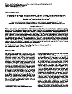
The solution is best represented in Figure 1, where the investment decision is mapped out in a two-dimensional space along the level of corruption in the host country and the level of technological sophistication of the investing firm. When corruption level q is sufficiently high, no foreign investment in any ownership form would take place. Conditional on foreign investment taking place, the foreign investor would prefer a wholly-owned form if its technology is sufficiently sophisticated. On the other hand, holding the level of technological sophistication constant, the higher the corruption (up to a limit), the more inclined the foreign investor is to set up a joint venture. Foreign Investor’s technological leadership Index

Vwo c+θ

tj

No Whollyowned Firms

FDI

Joint Ventures

0

Vwo − V JV θ

V JV C

Corruption in host country

qk

Figure 1: FDI Decision as a function of local corruption and firm’s technology

5

III. Empirical Evidence In this section, we report the statistical evidence on the connection between corruption and ownership structure of foreign direct investment. We describe the empirical work in three steps: (1) the economic specification, (2) some key variables (their measures and sources, with more details in a separate appendix), and (3) the regression results and their interpretations. Econometric Specification While using the simple theoretical model in the previous section to motivate our econometric specification, we also bring in additional control variables that the literature on foreign investment suggests are important. More specifically, we estimate a system consisting of two parts. The first part describes the investor’s decision to enter a particular host country, k. The second part describes the decision on the choice between wholly-owned form or joint venture, conditional on FDI taking place. Let FDIjk be a dummy variable that takes the value of one if firm j chooses to invest in host country k, and zero otherwise. We assume that this investment takes place if and only if a latent variable, FDI*jk is positive. The latent variable depends on a vector of factors including the level of corruption in host country k, denoted by qk. In other words,

FDI jk = 1 if FDI *jk > 0 FDI jk = 0 otherwise where FDI *jk = x jk β + γqk + ε kj X jk ≡ vector of determinants of FDI* other than corruption, and β (vector) and γ are

parameters. In subsequent discussion and in the regression tables, we label the last equation on FDI* as the “FDI decision equation.” Let OWNERSHIP jk be a dummy variable that takes the value of one if the foreign investment by firm j takes the wholly-owned form in host country k (conditional on the investment taking place), and zero if the investment is a joint venture. Wholly-owned form occurs if and only if another latent variable, OWNERSHIP*jk, is positive. In other words,

6

OWNERSHIP jk = 1 if OWNERSHIP *jk > 0 and FDI * jk > 0 OWNERSHIP jk = 0 if OWNERSHIP *jk ≤ 0 and FDI * jk > 0 where OWNERSHIP *jk = W jkθ + δ 1q k + δ 2t j + υ kj t j is an index of technological sophistication for firm j, W is a vector of determinants of the ownership structure other than host country’s corruption and foreign investor’s technological sophistication, θ (vector), δ 1 and δ 2 are parameters to be estimated. In subsequent discussion and in the regression tables, we label the last equation on OWNERSHIP* as the “ownership decision equation.” Assuming that (ε, ν) are i.i.d normal variables with zero means and a correlation coefficient of ρ, we estimate these equations (probit with sample selection) simultaneously by maximum likelihood. The number of observations in the FDI decision equation is equal to the number of firms in the sample, multiplied by the number of destination countries in the sample. In the ownership decision equation, the number of observations is equal to the total number of (actual or planned) FDI projects in the sample. In terms of the parameterization described above, the central hypotheses that we seek to test are the following: (a) Corruption discourages foreign direct investment, i.e., γ < 0, in the FDI decision equation; (b) Conditional on FDI taking place and holding constant the technological level of the foreign investor, corruption encourages the joint venture form (or discourages the sole ownership), i.e., δ 1 < 0, in the ownership decision equation; And (c) conditional on FDI taking place, a more technologically advanced firm is more likely to adopt a wholly-owned form, i.e., δ 2 > 0 in the ownership decision equation.

Data Our empirical work employs a unique firm-level data set based on a survey conducted by the European Bank for Reconstruction and Development. In January 1995, a brief questionnaire was sent out to all companies (about 9,500) listed in the Worldscope database. 6 6

Worldscope is a commercial database that provides detailed financial statements, business descriptions, and historical pricing information on thousands of public companies located in more than fifty countries.

7

Responses were obtained from 1,405 firms that answered questions regarding their existing or planned FDI in Eastern Europe and the former Soviet Union. 7 381 respondents had actually invested and further 70 firms planned to invest in the region. The survey inquired about the form of the project: a joint venture with a local partner, acquisition or greenfield. For the purposes of this study, we treat all projects not associated with JVs as wholly owned. The questionnaire did not ask for the exact ownership shares between foreign and local partners for joint ventures, nor the timing nor the size of the investment, which are unfortunate for us. Since inflows of FDI were negligible prior to 1989, the investments covered in our sample took place (or were planed to take place) between 1989 and 1995. 8 Table 1 presents the distribution of investment projects across host countries. A key regressor is host country’s corruption level. Corruption, by its very nature, is difficult to get a precise measure. There are a few measures available “on the market,” all of which are subjective perceptions 9 . There are three types of such indexes. The first is based on surveys of individual “experts” (typically every country is rated by one expert). Popular examples of this type include the Business International (BI) Index used in Mauro (1995), Wei (1997 and 2000) and others, and International Country Risk Group (ICRG) index used by, for example, Ades and Di Tella (1999) and Wei (2000). The second type is based on surveys of firms. Typically multiple firms per country are surveyed, and the average answer for each country is used as the value of corruption index for that country. Relative to the first type, this type of indexes reduces the impact of the idiosyncratic errors of individual respondents. Most popular indexes of this type include the Global Competitiveness Report (GCR) index by the World Economic Forum and the World Development Report (WDR) index by the World Bank. Both GCR and WDR indexes were used in Kaufmann and Wei (1999). The third type is to pool together information from several existing indexes by averaging or other statistical extraction methods. The most widely known index of this type is the one compiled by the Transparency International (TI), an international non-governmental

7

117 of the survey respondents were chosen for in-depth interviews whose results are discussed in Lankes and Venables (1996). 8 “Several CEECs had already allowed minority foreign participation in joint ventures in the 1970s and 1980s, but this opportunity was not attractive enough to foreign investors. Except for a few showpieces, foreign investment started to flow only after the transformation to market economy had been launched” (Hunya, 1997, p. 286). 9 See Wei (1999) for a discussion of the various corruption indexes.

8

organization dedicated to fighting corruption. 10 Unfortunately, many of these indexes such as the BI, GCR and ICRG indexes, do not cover enough transition economies to be useful for our examination. In this paper, we use two corruption indexes that have adequate coverage of the transition economies. The first one is the WDR index, which is based on a survey undertaken in 1996 by the World Bank in preparation of the World Development Report 1997. The survey covered 3,866 firms in 73 countries. The rating is based on the response to Question 14 which asked: “Is it common for firms in my line of business to have to pay some irregular, ‘additional’ payments to get things done?” The respondents were asked to rate corruption on a 1 to 6 scale with 1 denoting “always” and 6 “never.” To facilitate interpretation of the results we re-scaled the variable in the following way: re-scaled WDR index = 7 – original WDR index. Thus, higher values correspond to a higher level of corruption. The second measure is the 1999 Transparency International Corruption Perception Index (TI index for short) which pools information from ten different surveys of business executives, risk analysts and the general public. The original index ranges between 10 (highly clean) and 0 (highly corrupt). Again we re-scale the index so that a higher value corresponds to a higher level of corruption. 11 There is a regrettable mismatch in timing between our corruption measures (1996 and 1999, respectively) and the FDI data (1995). Unfortunately, as far as we know, all corruption indexes prior to 1995 do not cover most of the transition economies in our sample. We note however that the relative rankings of corruption levels across countries are unlikely to change very much in a five year span. For example, the International Country Risk Group (ICRG) corruption index covers eight countries in our sample. The Spearman rank correlation coefficients for these countries are 0.98 between the 1994 and 1996 values, and 0.94 between the 1994 and 1998 values, respectively. Hence, as far as these countries are concerned, the relative rankings are fairly stable in the 1990s. Nonetheless, the mismatch is a shortcoming that we need to keep in mind. Note also that our estimation would produce a negative sign on the corruption variable if corruption per se was not affecting the choice of entry mode but its level was positively 10

Kaufmann, Kraay and Zoido-Lobaton (1999) constructed their own index by pooling information from existing indexes using an unobserved component method.

9

correlated with the restrictions on the extent of foreign ownership. To the best of our knowledge, however, in none of the countries in the sample there exists legislation specifically forbidding full ownership by foreign investors. For instance, in the USSR a presidential decree issued as early as October 1990 allowed foreign wholly owned companies to be established in the form of branches or subsidiaries. The decree also created the legal basis for foreign investors to buy out existing Soviet enterprises as these were privatized (McMillan 1996, p. 50). In Hungary, Act XXIV of 1988 on the Investment of Foreigners in Hungary allowed non-Hungarian companies to own equity up to 100% (WTO, 1998). In Poland, the 1988 Law on Economic Activity with the Participation of Foreign Parties permitted 100 per cent foreign equity participation (GATT, 1992). In many transition economies, however, FDI in sectors such as production of military equipment and extraction of natural resources has been subject to restrictions on the extent of foreign ownership. 12 Therefore, we exclude firms in the coal, gas and oil industry from our sample. Since service sectors tend to be more restricted than manufacturing, we focus on firms in manufacturing sectors only. Another crucial variable in our regressions is a measure of investor’s technological sophistication. We use the ratio of firm R&D intensity to the industry average, as suggested by Smarzynska (2000). 13 We also include industry level R&D intensity. In addition to technology leakage, foreign investors may be concerned about dissipation of other intangible assets, for instance, marketing techniques. Thus, we also control for industry advertising intensity and investor’s sophistication in marketing techniques. The latter is proxied by investor’s advertising intensity relative to the industry mean. 14 All of these variables, with the exception of industry advertising intensity, were found by Smarzynska to be positively related to the probability of full ownership. Additionally, we control for firm size, production diversification and the distance between home and host countries. Blomström and Zejan (1991) suggested that larger firms 11

While an index corresponding to an earlier year would have been more appropriate, it covered a smaller number of countries in our data set. 12 See Dunning and Rojec (1993) for a description. 13 R&D intensity is defined as the ratio of R&D expenditure to net sales. The figures for R&D intensity and other firm specific variables come from the Worldscope database. See Appendix I for more details. 14 There is also another reason why firms investing heavily in advertising may want to seek full ownership. A JV partner may have a strong incentive to free ride on the reputation of a foreign partner by debasing the quality of

10

are more likely to take higher risks and thus more often choose full ownership. Their empirical results, however, led to the opposite conclusion. Stopford and Wells (1972) pointed out that more diversified firms may be more tolerant towards minority ownership and thus more likely to engage in JVs. Meyer (1998) has confirmed this prediction. Finally, we include a measure of the distance between investor’s home country and the investment destination as a proxy for cultural distance. As Kogut and Singh (1988) have shown, cultural distance is positively related to the probability of a JV which suggests that a local partner is more useful in less familiar environment. The investment equation includes several other regressors such as a host country’s GDP, GDP per capita, distance between investor’s country and the host as well as a measure of unit labor costs and tax rates in the host country. We expect to find that the probability of investment is positively related to the market size (GDP) and purchasing power of local consumers (GDP per capita) and negatively correlated with distance, labor costs and tax rates. Additionally, we control for production diversification since less diversified firms are more likely to be forced by competitive pressures in their home countries to search for new markets. 15 All variables are described in more detail in Appendix I. Summary statistics are listed in Table 1A in Appendix II.

Statistical Results Table 2 presents the estimation results using the WDR index as our measure of corruption. Column 1 reports the basic regression. The top panel describes the FDI decision equation. We find that foreign investors that are large and have a less diversified production structure are more likely to invest in the transition economies. They are attracted to countries with large markets and higher GDP per capita. Distance between investor’s country and the host has a negative impact on the probability of FDI. More essential for the current paper, we find that more corruption in a host country is associated with a lower probability of investment. The two interactive terms between host country corruption and foreign investor’s

the product carrying the foreign trademark. In such a case, the local partner appropriates the full benefits of debasement while bearing only a small fraction of the costs (Caves, 1982). 15 See Markusen (1995) for a survey of FDI determinants.

11

technological level are insignificant. The two interactive terms between host country corruption and the firm’s marketing intensity are positive and significant. In the lower panel of Column1, where the result on the ownership decision is reported, we find that the coefficient on corruption is negative and statistically significant, indicating that corruption encourages foreign investor to form a joint venture with a local partner, which is consistent with our hypothesis. The coefficients on measures of the foreign investor’s level of technological (and marketing) sophistication are positive and (mostly) significant, indicating that firms with better technology are more reluctant to use local partners, which is also consistent with our hypothesis. It may be interesting to see the magnitude of the effect of corruption on the ownership composition as estimated in Column 1. As corruption decreases from the level of Azerbaijan (WDR corruption index = 4.6 on a 1-7 scale) to that of Hungary (WDR corruption index = 2.6), the probability that a foreign investor will enter through a wholly-owned subsidiary goes up by fourteen percentage points (say from 30% to 44%). In Columns 2 and 3, we progressively add host country’s marginal corporate tax and unit labor cost to the FDI decision equation. We find that the tax rate is not significant in our sample, but low labor cost does help to attract FDI. As far as our key hypotheses are concerned, corruption continues to have a negative effect on FDI entry and on the likelihood of sole ownership, and high technological sophistication of the foreign investors still make them shy away from joint ventures. These are the same as the estimates in Column 1 16 . In Columns 4-6, we repeat the first three regressions except that we also add the distance (in log) between the host and source countries in the ownership decision equations. This is to examine the possibility that informational barriers that are correlated with the distance may encourage foreign investors to use a local partner. While the negative signs on the coefficients are consistent with this view, they are not statistically different from zero. Again, host country corruption continues to discourage inward FDI, and conditional on FDI taking place, continues to discourage sole ownership. In the FDI decision equations (top panel of Table 2), the interaction terms between corruption and technological sophistication do not appear to be statistically significant. 16

In Column 3, while the coefficient on corruption is still negative in the ownership decision equation, but the significance level drops to 15%. This is due to an increase in the standard error of the estimator rather than a decrease in the absolute value of the point estimate.

12

Interactions with marketing sophistication proxies bear positive and significant coefficients. This result suggests that marketing know-how does not affect investors’ decisions in the same way as technological sophistication. In regressions that are not reported here, we have also experimented with including the interactive terms between firms’ technological sophistication and host country corruption in the ownership decision equations. If we do not include the measures of technological level by themselves, the coefficients on the interactive terms are positive and statistically significant. Corruption variable continues to have a negative and statistically significant coefficient in the ownership decision equation. This result can be consistent with the following hypothesis: foreign investors are generally more inclined to form joint ventures in a corrupt country, but their interest in joint ventures decreases with their level of technological sophistication because of the concern that intellectual property rights protection becomes more problematic in a more corrupt country. On the other hand, if both the interactive terms and the technology variables by themselves are included in the ownership decision equations, both sets of coefficients become statistically insignificant. This could be due to a multicollinearity problem. In any case, we are not able to say anything definitive about the interactive term between corruption and technological sophistication. In Table 3, we repeat the regressions in Table 2 by using the Transparency International index as an alternative measure of host country corruption. The results are essentially the same. In particular, we find that corruption discourages foreign investment in the first place. Once foreign investment takes place, corruption discourages wholly-owned foreign firms. As mentioned at the beginning of the paper, Hines (1995) suggests that US multinationals are more likely to avoid joint ventures in corrupt countries than investors of other nationalities. To test this hypothesis, we include in both equations of our model a dummy variable for US investors and an interaction between the dummy and corruption level. The results are presented in Table 4. We find no evidence that American firms invest less in corrupt countries, which is consistent with the results of Wei (2000). We show, however, that US companies are indeed more averse to joint ventures in more corrupt host countries (or more likely to set up wholly-owned firms). The last finding may be due to the Foreign Corrupt Practices Act of 1977.

13

IV. Conclusions This paper studies how a foreign investor’s choice of the entry mode is affected by both the investor’s technological sophistication and the extent of corruption in a host country. Corruption makes local bureaucracy less transparent and hence increases the value of a local joint venture partner to a foreign investor. On the other hand, foreign investors with sophisticated technology may worry about leakage of technological know-how by joint venture partners and are thus less inclined to form a joint venture. We test these hypotheses using a firm-level data se on FDI in Eastern Europe and the Former Soviet Union in the early 1990s. The data are broadly consistent with our hypotheses. In addition, we find that, other things equal, American investors are somewhat more reluctant to form joint ventures in more corrupt countries, possibly because of the U.S. Foreign Corrupt Practices Act of 1977. For joint venture firms, our data set does not have information on the exact ownership shares between foreign and local partners. It may be useful to work out the effect of corruption on majority- versus minority-owned joint ventures and test it with some more refined data in the future.

References Ades, Alberto, and Rafael Di Tella, 1999, “Rents, Competition, and Corruption,” American Economic Review. 89(4): 982-993. Asiedu, Elizabeth and Hadi Salehi Esfahani, 1998, “Ownership Structure in Foreign Direct Investment Projects” CIBER Working Paper No. 98-108. Blomström, Magnus and Mario Zejan, 1991, “Why Do Multinational Firms Seek Out Joint Ventures?” Journal of International Development. 3(1): 53-63. Caves, R., 1982, Multinational Enterprise and Economic Analysis. Cambridge University Press: New York. Dunning, John H and Matija Rojec, 1993, Foreign Privatization in Central & Eastern Europe. CEEPN: Ljubljana, Slovenia. Froot, Kenneth, 1993, Foreign Direct Investment, Chicago: University of Chicago Press. GATT, 1992, Trade Policy Review: Poland. Geneva. Vol. 1. Havlik, Peter, 1996, “Exchange rates, competitiveness and labour costs in Central and Eastern Europe,” WIIW Research Report No. 231 (WIIW, Vienna). Hines, James R. Jr., 1995, “Forbidden Payment: Foreign Bribery and American Business After 1977” NBER Working Paper 5266.

14

Hunya, Gabor, 1997, Large privatisation, restructuring and foreign direct investment in: Salvatore Zecchini, ed., Lessons from the economic transition. Central and Eastern Europe in the 1990s (Kluwer Academic Publishers, Dordrecht, Boston and London): 275-300. Kaufmann, Daniel, Aart Kraay, and Pablo Zoido-Lobaton, 1999, “Aggregating Governance Indicators.” World Bank working paper. Kaufmann, Daniel, and Shang-Jin Wei, 1999, “Does ‘Grease Payment’ Speed Up the Wheels of Commerce?” NBER Working Paper 7093, April. Also released as a World Bank Policy Research Working Paper 2254. Kogut, Bruce and Harbir Singh, 1988, “The Effect of National Culture on the Choice of Entry Mode,” Journal of International Business Studies. 19: 411-432. Lankes, Hans-Peter and Anthony J. Venables, 1996, “Foreign direct investment in economic transition: The changing pattern of investments,” Economics of Transition. 4: 331347. Markusen, James R., 1995, The boundaries of multinational enterprises and the theory of international trade, Journal of Economic Perspectives. 9: 169-189. Mauro, Paolo, 1995, “Corruption and Growth,” Quarterly Journal of Economics, 110: 681712. McMillan, Carl H., 1996, “Foreign Investment in Russia: Soviet Legacies and Post-Soviet Prospects” in Patrick Artisien-Maksimenko and Yuri Adjubei, eds. Foreign Investment in Russia and Other Soviet Successor States. St. Martin’s Press, Inc.: New York: 4172. Meyer, Klaus E., 1998, Direct Investment in Economies in Transition. Edward Elgar: Cheltenham, UK and Northampton, MA. Pearce, E.A. and C.G. Smith, 1984, The World Weather Guide, London: Hutchinson. Rudloff, Willy, 1981, World Climates, with tables of climatic data and practical suggestions, Stuffgart: Wissenschaftliche Verlagsgesellschaft. Smarzynska, Beata K., 2000, “Technology Transfer and Foreign Investors’ Choice of Entry Mode” The World Bank Policy Research Working Paper. Forthcoming. Stopford, John M. and Louis T. Wells, Jr., 1972, Managing the Multinational Enterprise. Basic Books, Inc.: New York. Wei, Shang-Jin, 1997, “Why is Corruption So Much More Taxing Than Taxes? Arbitrariness Kills, “ National Bureau of Economic Research Working Paper 6255, November. Wei, Shang-Jin, 1998, “Corruption and Economic Development in Asia,” in Integrity in Governance in Asia, edited by the United Nations Development Program, New York: UNDP. Wei, Shang-Jin, 2000, "How Taxing is Corruption on International Investors?" Review of Economics and Statistics. 82 (1): 1-11.

15

Wheeler, David and Ashoka Mody, 1992, “International Investment Location Decisions: The Case of US Firms,” Journal of International Economics 33:57-76. WTO, 1998, Trade Policy Review: Hungary. Geneva.

16

Appendix I Firm specific variables used in the empirical analysis come from Worldscope which is a commercial database providing detailed financial statements, business descriptions, and historical pricing information on thousands of public companies located in more than fifty countries. They pertain to 1993 or the closest year for which the information was available and refer to worldwide operations of each firm. Below we present a more detailed description of the variables. Ø Industry R&D intensity: measured by R&D expenditure as a percentage of net sales. To find the industry averages we used figures for all firms listed in Worldscope in a given industry. The industry averages have been calculated at the three digit SIC industry classification17 Ø Relative R&D intensity: measured by the ratio of a firm’s R&D intensity to the industry average 18 Ø Industry advertising intensity: measured by Sales, General and Administrative expenditure divided by net sales. This variable is a standard proxy for advertising intensity used in the literature Ø Relative advertising intensity: measured by the ratio of a firm’s advertising intensity to the industry average Ø Firm size: measured by a firm’s sales in millions of US dollars Ø Diversification: measured by the number of four digit SIC codes describing a firm’s activities Ø GDP and GDP per capita: data for 1993. Source: EBRD (1994) Ø Corruption WDR: WDR rating is based on the response to question 14 which asked: “Is it common for firms in my line of business to have to pay some irregular, “additional” payments to get things done?” The respondents were asked to rate corruption on a 1 to 6 17

When calculating industry averages, we have removed two outliers from the drug sector and one from communications equipment industry. These firms reported R&D intensities equal to 16598, 1815 and 2560, respectively. All three firms reported sales below $500,000 thus they are likely to be start up companies. Note that the conclusions of the paper are remain unchanged even if this correction is not performed. 18 If firm and industry level figures were both equal to zero, relative R&D intensity took on the value of one.

17

scale with 1 denoting “always” and 6 “never.” To facilitate interpretation of the results we rescaled the variable in the following way: rescaled WDR = 7 – original WDR. Thus, higher values correspond to a higher level of corruption Ø Corruption TI: Transparency International Corruption Perceptions Index relates to perceptions of the degree of corruption as seen by business people, risk analysts and the general public. It ranges between 10 (highly clean) and 0 (highly corrupt). Again we rescaled the index so that higher values correspond to a higher level of corruption. Rescaled TI index = 11 – original TI index Ø Distance: logarithm of distance in kilometers between the capital cities. The primary source is Rudloff (1981), supplemented by Pearce and Smith (1984). In the case of following countries the average distance from the main cities was used: Argentina (Buenos Aires, Cordoba, Rosario), Australia (Canberra, Sydney, Melbourne), Canada (Toronto, Vancouver, Montreal), Russia (Moscow, St. Petersburg, Nizhni Novogorod). The data for Nizhni Novogorod is from http://www.unn.runnet.ru/nn/whereis.htm. For the United States Kansas City, Missouri was used, for Netherlands De Bilt, Slovakia Poprad, Switzerland Zurich. Distances between Taiwan and other countries are from Shang-jin Wei’s NBER web site: www.nber.org/~wei. Ø Unit labor costs: relative to the Austrian level. Source: Havlik (1996) Ø Corporate tax rate: in percentages; if several rates apply, the highest one was used. Source: PriceWaterhousePaineWebber. Distance, GDP, GDP per capita and firm size are used in the log form.

18

Table 1. Distribution of Projects by Host Country Host country Albania Azerbaijan Belarus Bulgaria Croatia Czech Estonia FYR Macedonia Georgia Hungary Kazakhstan Latvia Lithuania Moldova Poland Romania Russia Slovakia Slovenia Turkmenistan Ukraine Uzbekistan TOTAL

No of JV projects in the sample

No. of wholly owned projects in the sample

3 1 5 16 7 55 16 2 4 50 10 13 8 2 84 21 83 26 13 1 20 5 445

1 1 3 13 4 53 8 1 2 48 6 6 5 0 51 12 31 19 5 0 5 1 275

Total no. of projects in the sample

4 2 8 29 11 108 24 3 6 98 16 19 13 2 135 33 114 45 18 1 25 6 720

Source countries (listed in the decreasing order of importance in the sample): Germany, United Kingdom, France, United States, Finland, Sweden, Switzerland, Netherlands, Denmark, Norway, Belgium, Australia, Japan, Austria, Portugal, Canada, Greece, Italy, Ireland, Brazil, Spain, Singapore, Malaysia, South Africa and South Korea.

19

Table 2. Corruption and Ownership Structure of FDI: WDR Corruption Index FDI DECISION EQUATION -4.1270** -5.2929** -4.0330** -4.1160** -5.1227** (0.5720) (0.8722) (0.5693) (0.5737) (0.8698) Firm size 0.2282** 0.2397** 0.2281** 0.2283** 0.2397** (0.0202) (0.0226) (0.0202) (0.0203) (0.0226) Production Diversification -0.0301* -0.0189 -0.0306* -0.0302# -0.0190 (0.0184) (0.0212) (0.0183) (0.0184) (0.0212) Total GDP 0.3604** 0.3530** 0.3663** 0.3606** 0.3492** (0.0269) (0.0426) (0.0267) (0.0268) (0.0426) GDP per capita 0.0573 0.1732** 0.0561 0.0562 0.1694** (0.0544) (0.0830) (0.0541) (0.0545) (0.0828) WDR Corruption Index -0.3515** -0.3899** -0.3302** -0.3519** -0.3990** (0.0768) (0.1011) (0.0736) (0.0768) (0.0997) Firm Tech Sophistication 0.0063 0.0065 0.0063 0.0063 0.0066 * WDR Corruption Index (0.0090) (0.0103) (0.0091) (0.0091) (0.0104) Industry Tech Sophistication -0.0026 -0.0028 -0.0027 -0.0026 -0.0028 * WDR Corruption Index (0.0034) (0.0042) (0.0034) (0.0034) (0.0042) Firm Marketing Sophist. 0.0557** 0.0758** 0.0555** 0.0557** 0.0755** * WDR Corruption Index (0.0196) (0.0210) (0.0197) (0.0197) (0.0211) Industry Marketing Sophist. 0.0044** 0.0046** 0.0044** 0.0044** 0.0045** * WDR Corruption Index (0.0008) (0.0009) (0.0008) (0.0008) (0.0009) Distance -0.4850** -0.3988** -0.4892** -0.4854** -0.4015** (0.0369) (0.0454) (0.0372) (0.0372) (0.0454) Tax rate 0.0060 0.0004 0.0059 -0.0005 (0.0056) (0.0067) (0.0056) (0.0067) Unit labor cost -0.0115* -0.0123* (0.0066) (0.0066) OWNERSHIP DECISION EQUATION Constant -2.8361** -2.8050** -3.3824** -2.7816** -2.7600** -3.1644** (0.9607) (0.9642) (1.2055) (0.9892) (0.9926) (1.1121) Firm size 0.1428** 0.1416** 0.1780** 0.1483** 0.1463** 0.2152** (0.0496) (0.0498) (0.0552) (0.0521) (0.0524) (0.0530) Production Diversification -0.1063** -0.1068** -0.0929** -0.1078** -0.1080** -0.0974** (0.0419) (0.0419) (0.0443) (0.0423) (0.0424) (0.0437) Firm Tech Sophistication 0.1986** 0.1980** 0.1647** 0.1970** 0.1967** 0.1594** (0.0662) (0.0663) (0.0767) (0.0673) (0.0673) (0.0754) Industry Tech Sophistication 0.1290** 0.1289** 0.1018** 0.1283** 0.1283** 0.0939** (0.0302) (0.0302) (0.0320) (0.0302) (0.0302) (0.0317) Firm Marketing Sophist. 0.7116** 0.7103** 0.7305** 0.7136** 0.7122** 0.7312** (0.1667) (0.1669) (0.1811) (0.1656) (0.1660) (0.1668) Industry Marketing Sophist. 0.0052 0.0051 0.0102 0.0053 0.0052 0.0115# (0.0070) (0.0070) (0.0076) (0.0070) (0.0070) (0.0072) WDR Corruption Index -0.2306* -0.2278* -0.2463# -0.2242* -0.2224* -0.2238# (0.1308) (0.1314) (0.1524) (0.1347) (0.1353) (0.1482) Distance -0.0252 -0.0213 -0.1468 (0.0962) (0.0964) (0.1250) Rho (1,2) 0.1151 0.1041 0.1451 0.1424 0.1275 0.3897 (0.1656) (0.1665) (0.2414) (0.1876) (0.1889) (0.2784) No Obs Eq1 6004 6004 2212 6004 6004 2212 No Obs Eq2 339 339 282 339 339 282 Log L -1074.10 -1073.505 -827.9399 -1074.062 -1073.477 -827.2233 **, *, # denote significant at 5%, 10% and 15% level, respectively. Standard errors are presented in parentheses. GDP, GDP per capita, distance and firm size are in logarithms. Constant

-4.0457** (0.5673) 0.2281** (0.0201) -0.0306* (0.0183) 0.3661** (0.0267) 0.0574 (0.0540) -0.3295** (0.0736) 0.0063 (0.0090) -0.0027 (0.0033) 0.0555** (0.0195) 0.0044** (0.0008) -0.4888** (0.0368)

20

Table 3. Using TI Corruption Index FDI DECISION EQUATION -2.4314** -3.0539** -2.4355** -2.4353** -3.0380** (0.7128) (1.0812) (0.7136) (0.7146) (1.0780) Firm size 0.2205** 0.2319** 0.2205** 0.2205** 0.2318** (0.0189) (0.0212) (0.0189) (0.0189) (0.0212) Production Diversification -0.0388** -0.0338* -0.0387** -0.0388** -0.0338* (0.0172) (0.0197) (0.0173) (0.0173) (0.0198) Total GDP 0.4489** 0.4842** 0.4494** 0.4489** 0.4836** (0.0308) (0.0428) (0.0306) (0.0308) (0.0429) GDP per capita -0.1812** 0.0361 -0.1854** -0.1810** 0.0363 (0.0742) (0.0938) (0.0724) (0.0745) (0.0939) TI Corruption Index -0.2406** -0.4332** -0.2478** -0.2406** -0.4332** (0.0553) (0.0786) (0.0523) (0.0553) (0.0787) Firm Tech Sophistication 0.0034 0.0040 0.0034 0.0034 0.0040 * TI Corruption Index (0.0041) (0.0046) (0.0041) (0.0041) (0.0046) Industry Tech Sophistication -0.0011 -0.0007 -0.0011 -0.0011 -0.0007 * TI Corruption Index (0.0015) (0.0018) (0.0016) (0.0016) (0.0019) Firm Marketing Sophist. 0.0236** 0.0312** 0.0236** 0.0236** 0.0312** * TI Corruption Index (0.0088) (0.0095) (0.0088) (0.0088) (0.0096) Industry Marketing Sophist. 0.0020** 0.0021** 0.0020** 0.0020** 0.0021** * TI Corruption Index (0.0003) (0.0004) (0.0003) (0.0003) (0.0004) Distance -0.4794** -0.4023** -0.4782** -0.4792** -0.4025** (0.0342) (0.0414) (0.0347) (0.0347) (0.0417) Tax rate -0.0023 -0.0045 -0.0023 -0.0047 (0.0055) (0.0063) (0.0055) (0.0063) Unit labor cost -0.0311** -0.0312** (0.0060) (0.0061) OWNERSHIP DECISION EQUATION Constant -2.3198** -2.3351** -2.4562* -2.3368** -2.3501** -2.4278* (0.9995) (0.9993) (1.2743) (1.0125) (1.0115) (1.2519) Firm size 0.1302** 0.1306** 0.1506** 0.1261** 0.1270** 0.1622** (0.0477) (0.0476) (0.0535) (0.0521) (0.0521) (0.0620) Production Diversification -0.0935** -0.0933** -0.0839** -0.0922** -0.0922** -0.0873** (0.0409) (0.0409) (0.0423) (0.0419) (0.0419) (0.0436) Firm Tech Sophistication 0.2120** 0.2122** 0.1796** 0.2130** 0.2132** 0.1788** (0.0644) (0.0645) (0.0735) (0.0650) (0.0651) (0.0735) Industry Tech Sophistication 0.1238** 0.1239** 0.0996** 0.1243** 0.1243** 0.0982** (0.0297) (0.0297) (0.0315) (0.0297) (0.0296) (0.0315) Firm Marketing Sophist. 0.7693** 0.7698** 0.7691** 0.7673** 0.7681** 0.7765** (0.1624) (0.1624) (0.1784) (0.1633) (0.1632) (0.1765) Industry Marketing Sophist. 0.0078 0.0079 0.0117# 0.0077 0.0078 0.0120* (0.0068) (0.0068) (0.0072) (0.0068) (0.0068) (0.0072) TI Corruption Index -0.1726** -0.1728** -0.1843** -0.1772** -0.1769** -0.1737** (0.0659) (0.0659) (0.0743) (0.0723) (0.0726) (0.0851) Distance 0.0177 0.0158 -0.0462 (0.0984) (0.0990) (0.1360) Rho (1,2) 0.0813 0.0858 0.0274 0.0621 0.0686 0.0883 (0.1522) (0.1520) (0.1986) (0.1819) (0.1823) (0.2680) No Obs Eq1 6636 6636 3160 6636 6636 3160 No Obs Eq2 361 361 306 361 361 306 Log L -1193.945 -1193.859 -941.809 -1193.926 -1193.844 -941.7314 **, *, # denote significant at 5%, 10% and 15% level, respectively. Standard errors are presented in parentheses. GDP, GDP per capita, distance and firm size are in logarithms. Constant

-2.4312** (0.7120) 0.2205** (0.0188) -0.0387** (0.0172) 0.4493** (0.0305) -0.1856** (0.0721) -0.2479** (0.0522) 0.0034 (0.0041) -0.0011 (0.0015) 0.0236** (0.0088) 0.0020** (0.0003) -0.4783** (0.0342)

21

Table 4. Are US Investors Special? FDI DECISION EQUATION Constant Firm size Production Diversification Total GDP GDP per capita Corruption Firm Tech Sophistication * Corruption Industry Tech Sophist. * Corruption Firm Marketing Sophist. * Corruption Industry Marketing Sophist. * Corruption Distance

WDR -2.5416** (0.6213) 0.2197** (0.0204) -0.0082 (0.0190) 0.3819** (0.0277) 0.0289 (0.0558) -0.3138** (0.0814) 0.0048 (0.0097) -0.0017 (0.0035) 0.0610** (0.0200) 0.0046** (0.0008) -0.7073** (0.0530)

WDR -2.5925** (0.6295) 0.2199** (0.0205) -0.0081 (0.0191) 0.3790** (0.0278) 0.0291 (0.0560) -0.3249** (0.0855) 0.0048 (0.0097) -0.0017 (0.0035) 0.0610** (0.0200) 0.0046** (0.0008) -0.7033** (0.0535) 0.0028 (0.0058)

0.4779 (0.4725) 0.0837 (0.1312)

0.4643 (0.4759) 0.0857 (0.1317)

Tax rate

WDR -3.1373** (0.9754) 0.2332** (0.0228) -0.0039 (0.0220) 0.3724** (0.0445) 0.1355# (0.0847) -0.4141** (0.1174) 0.0054 (0.0113) -0.0024 (0.0044) 0.0795** (0.0216) 0.0047** (0.0009) -0.6637** (0.0739) -0.0036 (0.0071) -0.0115* (0.0067) 0.1122 (0.5406) 0.2020 (0.1515)

Unit labor cost US parent US parent * Corruption

TI -1.0293 (0.7548) 0.2117** (0.0191) -0.0193 (0.0179) 0.4598** (0.0319) -0.1978** (0.0746) -0.2099** (0.0540) 0.0027 (0.0044) -0.0008 (0.0016) 0.0257** (0.0090) 0.0021** (0.0004) -0.7190** (0.0509)

TI -1.0150 (0.7540) 0.2115** (0.0191) -0.0193 (0.0179) 0.4590** (0.0321) -0.1878** (0.0763) -0.1924** (0.0579) 0.0026 (0.0044) -0.0008 (0.0016) 0.0257** (0.0090) 0.0021** (0.0004) -0.7246** (0.0514) -0.0053 (0.0056)

1.0451* (0.5674) -0.0332 (0.0752)

1.0700* (0.5721) -0.0354 (0.0756)

TI -1.1330 (1.1652) 0.2247** (0.0213) -0.0215 (0.0205) 0.4973** (0.0446) 0.0074 (0.0964) -0.4014** (0.0841) 0.0035 (0.0050) -0.0007 (0.0019) 0.0324** (0.0097) 0.0022** (0.0004) -0.6795** (0.0692) -0.0079 (0.0066) -0.0300** (0.0061) 0.8617 (0.6125) -0.0068 (0.0808)

-1.3511 (1.1202) 0.1251** (0.0525) -0.0841** (0.0427) 0.2255** (0.0669) 0.1284** (0.0308) 0.7858** (0.1676) 0.0084 (0.0069) -0.2127** (0.0852) -0.1008 (0.1473) -1.6074 (1.4949) 0.2872# (0.1956) 0.0342 (0.1950) 6636 361 -1165.508

-0.8541 (1.5168) 0.1674** (0.0609) -0.0851* (0.0437) 0.1900** (0.0756) 0.0989** (0.0329) 0.7991** (0.1788) 0.0128* (0.0072) -0.2212** (0.0998) -0.2463 (0.2354) -1.5182 (1.6414) 0.2877 (0.2099) 0.0924 (0.2707) 3160 306 -920.4021

OWNERSHIP DECISION EQUATION Constant Firm size Production Diversification Firm Tech Sophistication Industry Tech Sophist. Firm Marketing Sophist. Industry Marketing Sophist. Corruption Distance US parent US parent * Corruption Rho (1,2) No Obs Eq1 No Obs Eq2 Log L

-1.6977# (1.1177) 0.1400** (0.0534) -0.0975** (0.0436) 0.2094** (0.0687) 0.1341** (0.0314) 0.7479** (0.1731) 0.0060 (0.0071) -0.2839* (0.1582) -0.1474 (0.1395) -1.4039 (1.2236) 0.5781* (0.3391) 0.0658 (0.2053) 6004 339 -1048.989

-1.6903# (1.1182) 0.1391** (0.0535) -0.0977** (0.0436) 0.2092** (0.0687) 0.1341** (0.0314) 0.7472** (0.1732) 0.0059 (0.0071) -0.2833* (0.1584) -0.1453 (0.1400) -1.4067 (1.2243) 0.5784* (0.3392) 0.0592 (0.2059) 6004 339 -1048.866

-1.2662 (1.4915) 0.2099** (0.0553) -0.0935** (0.0449) 0.1698** (0.0790) 0.0988** (0.0335) 0.7670** (0.1745) 0.0120# (0.0074) -0.3321* (0.1811) -0.3629* (0.2157) -1.2213 (1.3600) 0.5696# (0.3683) 0.3258 (0.3060) 2212 282 -807.5265

22

-1.3291 (1.1211) 0.1231** (0.0527) -0.0843** (0.0427) 0.2251** (0.0667) 0.1283** (0.0308) 0.7840** (0.1679) 0.0083 (0.0069) -0.2136** (0.0850) -0.0952 (0.1469) -1.6130 (1.4956) 0.2872# (0.1955) 0.0198 (0.1951) 6636 361 -1165.932

Appendix Table 1A. Summary Statistics Variable

No of obs.

Mean

Std. Dev.

GDP

21

19,651

38,812

GDP per capita

21

1,321

1,422

WDR Corruption Index

18

3.7

0.7

TI Corruption Index

20

7.6

1.2

Corporate tax rate

21

29.5

6.5

Unit labor cost

10

27.5

13.8

Distance

15,824

4,946

3,966

Firm size (all)

1,306

2,864,259

9,434,850

399

4,179,212

11,900,000

1,316

3.6

2.0

Production diversification (investors)

402

4.3

2.1

Relative R&D intensity (all)

523

1.3

2.5

Relative R&D intensity (investors)

195

1.7

3.5

1,045

2.1

3.0

Industry R&D intensity (investors)

355

2.3

3.1

Relative advertising intensity (all)

705

1.0

0.8

Relative advertising intensity (investors)

242

1.0

0.7

1,086

21.9

14.8

364

22.8

16.4

Firm size(investors) Production diversification (all)

Industry R&D intensity (all)

Industry advertising intensity (all) Industry advertising intensity (investors)

23