CONTROVERSY TREND DETECTION IN SOCIAL MEDIA

A Thesis Submitted to the Graduate Faculty of the Louisiana State University and Agricultural and Mechanical College in partial fulfillment of the requirements for the degree of Master of Science in The Interdepartmental Program in Engineering Science

by Rajshekhar V. Chimmalgi B.S., Southern University, 2010 May 2013

To my parents Shobha and Vishwanath Chimmalgi.

ii

Acknowledgments Foremost, I would like to express my sincere gratitude to my advisor Dr. Gerald M. Knapp for his patience, guidance, encouragement, and support. I am grateful for having him as an advisor and having faith in me. I would also like to thank Dr. Andrea Houston and Dr. Jianhua Chen for serving as members of my committee. I would like to thank Dr. Saleem Hasan, for his guidance and encouragement, for pushing me to pursue graduate degree in Engineering Science under Dr. Knapp. I would like to thank my supervisor, Dr. Suzan Gaston, for her encouragement and support. I also thank my good friends, Devesh Lamichhane, Pawan Poudel, Sukirti Nepal, and Gokarna Sharma for their input and supporting me through tough times. I would also like to thank all the annotators for their time and effort to help me annotate the corpus for this research. And thanks to my parents, brother, and sister for their love and support.

iii

Table of Contents Acknowledgments.......................................................................................................................... iii List of Tables .................................................................................................................................. v List of Figures ................................................................................................................................ vi Abstract ......................................................................................................................................... vii Chapter 1: Introduction ................................................................................................................... 1 1.1 Problem Statement ................................................................................................................ 1 1.2 Objectives .............................................................................................................................. 3 Chapter 2: Literature Review .......................................................................................................... 4 2.1 Motivation to Participate in Social Media............................................................................. 4 2.2 Trend Detection ..................................................................................................................... 4 2.3 Sentiment Analysis ................................................................................................................ 9 2.4 Controversy Detection......................................................................................................... 10 2.5 Corpora ................................................................................................................................ 11 Chapter 3: Methodology ............................................................................................................... 13 3.1 Data Collection .................................................................................................................... 13 3.1.1 Annotation .................................................................................................................... 16 3.1.2 Preprocessing ................................................................................................................ 17 3.2 Controversy Trend Detection .............................................................................................. 18 Chapter 4: Results and Analysis ................................................................................................... 20 4.1 Controversy Corpus............................................................................................................. 20 4.2 Controversy Trend Detection .............................................................................................. 22 4.2.1 Feature Analysis ........................................................................................................... 22 4.2.2 Classification Model Performance ............................................................................... 23 4.2.3 Discussion ........................................................................................................................ 30 Chapter 5: Conclusion and Future Research ................................................................................. 32 References ..................................................................................................................................... 33 Appendix A: Wikipedia List of Controversial Issues ................................................................... 37 Appendix B: IRB Forms ............................................................................................................... 44 Appendix C: Annotator’s Algorithm ............................................................................................ 46 Vita................................................................................................................................................ 47

iv

List of Tables Table 1: Data elements returned by the Disqus API ..................................................................... 15 Table 2: Interpretation of Kappa ................................................................................................... 21 Table 3: Feature ranking ............................................................................................................... 22 Table 4: Performance comparison between different classifiers at six hours ............................... 23 Table 5: Classification after equal class sample sizes .................................................................. 24 Table 6: Confusion matrix of classification after equal class sample sizes .................................. 25 Table 7: Classification .................................................................................................................. 26 Table 8: Confusion Matrix ............................................................................................................ 27 Table 9: Classification after equal class sample sizes .................................................................. 29 Table 10: Confusion matrix of classification after equal class sample sizes ................................ 30

v

List of Figures Figure 1: Data collection ............................................................................................................... 14 Figure 2: Example of comments returned by the Disqus API ...................................................... 14 Figure 3: Database ERD ............................................................................................................... 15 Figure 4: Definition of controversy .............................................................................................. 16 Figure 5: Example of the annotation process ................................................................................ 17 Figure 6: Pseudocode for calculating controversy score and post rate ......................................... 19 Figure 7: F-Score calculation ........................................................................................................ 20 Figure 8: Distribution of comments .............................................................................................. 22

vi

Abstract In this research, we focus on the early prediction of whether topics are likely to generate significant controversy (in the form of social media such as comments, blogs, etc.). Controversy trend detection is important to companies, governments, national security agencies, and marketing groups because it can be used to identify which issues the public is having problems with and develop strategies to remedy them. For example, companies can monitor their press release to find out how the public is reacting and to decide if any additional public relations action is required, social media moderators can moderate discussions if the discussions start becoming abusive and getting out of control, and governmental agencies can monitor their public policies and make adjustments to the policies to address any public concerns. An algorithm was developed to predict controversy trends by taking into account sentiment expressed in comments, burstiness of comments, and controversy score. To train and test the algorithm, an annotated corpus was developed consisting of 728 news articles and over 500,000 comments on these articles made by viewers from CNN.com. This study achieved an average Fscore of 71.3% across all time spans in detection of controversial versus non-controversial topics. The results suggest that it is possible for early prediction of controversy trends leveraging social media.

vii

Chapter 1: Introduction Millions of bloggers participate in blogs by posting entries as well as writing comments expressing their opinions on various subjects, such as reviews on consumer products and movies, news, politics, etc. on social media website such as Twitter and Facebook, essentially providing a real-time view of opinions, intentions, activities, and trends of individuals and groups across the globe (Gloor et al., 2009). Recent surveys reveal that 32% of the nearly 250 million bloggers worldwide regularly give opinions on products and brands, 71% of active Internet users read blogs, and 70% of consumers trust opinions posted online by other consumers (Glass & Colbaugh, 2010). Contents created by bloggers may enable early detection of emerging issues, topics, and trends in areas of interest even before they are recognized by the main stream media (Colbaugh & Glass, 2011). Detecting emerging trends is of interest to businesses, journalists, and politicians, who want to extract useful information on a particular time series and to make it possible to forecast future events (Mahdavi et al., 2009). These trends, however, are buried in massive amounts of unstructured text contents, and can be difficult to extract using automation. For example, social media has been used in health care to estimate the spread of diseases. One such research conducted by Signorini et al. (2011) used Twitter to track rapidly-evolving public sentiment with respect to H1N1 or swine flu and to track and measure actual disease activity. They were able to estimate the influenza activity one to two week before Centers for Disease Control and Prevention (CDC). Emerging Trend Detection can assist CDC and other public health authorities in surveillance for emerging infectious diseases and public concerns. An emerging trend is a topic area that is growing in interest and utility over time in social media sites such as Twitter, Facebook, blogs, etc. The task of emerging trend detection (ETD) is to identify topics which were previously unseen and are growing in importance from a larger collection of textual data within a specific span of time (Kontostathis et al., 2003). A controversial trend is a popular topic which invokes confilicting sentiment or views (Choi et al., 2010). Controversy trend detection is important to companies, governments, national security agencies, and marketing groups so that they can identify which issues the public is having problems with and to develop strategies to remedy them. 1.1 Problem Statement For trend detection in social media, researchers have looked at burstiness of terms mentioned within a certain time span (Alvanaki et al., 2012; Cataldi et al., 2010; Heum et al., 2011; Jeonghee, 2005; Mathioudakis & Koudas, 2010; Reed et al., 2011). Cataldi et al. also considered authority of users in identifying trends. Others have looked at how a topic spreads in clusters of connected users (Budak et al., 2011; Glass & Colbaugh, 2010; Takahashi et al., 2011).

1

Sentiment analysis determines the sentimental attitude of a speaker or writer. Researchers have studied sentiment analysis using data from product reviews, blogs, and news articles, obtaining reasonable performances in identifying subjective sentences, determining their polarity values, and finding the holder of the sentiment found in a sentence (Kim & Hovy, 2006; Ku et al., 2006; Zhuang et al., 2006). Researchers have used sentiment lexicons consisting of words with positive and negative polarity in detection of controversy (Choi et al., 2010; Pennacchiotti & Popescu, 2010). Little research has been done specifically in detecting controversial trends in social media. Pennacchiotti and Popescu (2010) have considered disagreement about an entity (i.e. proper nouns) and the presence of explicit controversy terms in tweets to detect controversy in Twitter resulting in an average precision of 66%. Choi et al. (2010) defines a controversial issue as a concept that invokes conflicting sentiment or views. They focus on detecting potential controversial issues from a set of news articles about a topic by using a probabilistic method called known-item query generation method and determine if the detected phrase is controversial by checking if the sum of the magnitude of positive and negative sentiments is greater than an specified threshold and difference between them is less than a specified threshold value. They evaluate their methodology on a dataset consisting of 350 articles for 10 topics by selecting top 10 issue phrases for each topic and asking three users if the phrase is appropriate for a controversial issue or not achieving a precision of 83%. While Vuong et al. (2008) used disputes among Wikipedia contributors, where an article is constantly being edited in a circular manner by different contributors expressing their personal viewpoint getting a precision of 15%. A topic becomes popular if it is something that the public cares about or impacts them personally for example: cure for AIDS or Cancer, tax break for the middle class, tax the rich, free education, etc. (Deci & Ryan, 1987). For a controversial topic to become popular to the public, it should exhibit the following characteristics: - People like or dislike the topic and express extreme emotions – either they are for it or against it (Popescu & Pennacchiotti, 2010). - Most people consider the topic to be controversial (Popescu & Pennacchiotti, 2010). - People will share a topic which they strongly agree or disagree with (Takahashi et al., 2011). - Public opinion is usually close to an even split for or against the topic (Choi et al., 2010; Popescu & Pennacchiotti, 2010). This research focuses on the early prediction of whether topics are likely to generate significant controversy (in the form of social media such as comments, blogs, etc.). An algorithm is developed to predict controversial trends by taking into account sentiment expressed in comments, burstiness of comments, and controversy score. To train and test the algorithm, an annotated corpus was developed consisting of 728 news articles and comments made on those articles by viewers of CNN.com. The methodology predicts which articles are controversial or non-controversial and how early they can be predicted. 2

1.2 Objectives Following are the objectives of this research: 

  

Develop an improved algorithm to detect controversial trends incorporating new features such as number of ‘Likes’, number of threaded comments, positive sentiment count, negative sentiment count, and controversy score. Create an annotated corpus for training/testing of the algorithm. Implement the model in an application. Analyze the models performance.

3

Chapter 2: Literature Review 2.1 Motivation to Participate in Social Media Based on the theory of reasoned action, Hsu and Lin (2008) developed a model involving technology acceptance, knowledge sharing and social influence. They indicated that ease of use and enjoyment and knowledge sharing (altruism and reputation) were positively related to the attitude toward blogging. Social factors such as community identification and attitude towards blogging significantly influenced a blog participant’s intention to continue to use blogs. Blogging provides an easy way for a person to publish material on any topic they wish to discuss on the web. Blogging is an act of sharing, a new form of socialization. With a popular issue, a blog can attract tremendous attention and exert great influence on society, for example blogs describing the firsthand accounts of human rights violation and persecution of the Syrian people by the Assad regime. Deci and Ryan (1987) have done research incorporating intrinsic motivation such as perceived enjoyment involving the pleasure and satisfaction derived from performing a behavior, while extrinsic motivation emphasizing performing a behavior to achieve specific goals or rewards has been done by Vellerand (1997). The theory of reasoned action (Fishbein & Ajzen, 1975) advocates that a person’s behavior is predicted by their intentions and that the intentions are determined by the person’s attitude and subjective norm concerning his or her behavior. Social psychologists consider that knowledge sharing motivation has two complementary aspects – egoistic and altruistic. The egoistic motive was based on economic and social exchange theory. It includes economic rewards (Deci, 1975). Bock and Kim (2002) combined the theory of reasoned action and economic and social exchange theory to propose expected rewards, expected social associations, and expected contribution as the major determinants of an individual’s knowledge sharing attitudes. The altruistic motive, assumes that an individual is willing to increase the welfare of others and has no expectation of any personal returns resembling organization citizenship behavior. While bloggers provide knowledge, they expect others’ feedback, thus obtaining mutual benefit. Reputation, expected relationships, and trust are also likely to provide social rewards. 2.2 Trend Detection Many researchers have used burstiness of terms within a certain timespan in order to detect trending topics. Alvanaki et al. (2012) created EnBlogue system, which monitors web 2.0 streams such as blog postings, tweets, and RSS news feeds to detect sudden increase in popularity of a tags. Research at the University of Toronto have created TwitterMonitor, a system which detects trends over Twitter stream by first identifying keywords which suddenly appear in tweets at an unusually high rate and groups them into trends based on their cooccurrences (Mathioudakis & Koudas, 2010). Jeonghee (2005) utilizes temporal information 4

associated with documents in the streams and discover emerging issues and topics of interest and their change by detecting buzzwords in the documents. A candidate term is considered a buzzword, if its degree of concentration is higher than a given threshold. Goorha and Ungar (2010) describes a system that monitors news articles, blog posts, review sites, and tweets for mentions of items (i.e. product or company) of interest, extract 100 words around the items of interest them and determine which phrases are bursty. A phrase is determined to be bursting if the phrase has occurred more than a specified minimum number of times today or recently occurred more than a specified number of times, and increased by more than a specified percentage over its recent occurrence rate. A phrase is determined to be significant if it is mentioned frequently and is relatively unique to the product with which it is associated. Budak et al. (2011) in their study, propose two structure-based trend definitions. They identify coordinated trends as trends where the trendiness of a topic is characterized by the number of connected pairs of users discussing it and uncoordinated trends as trends where the score of a topic is based on the number of unrelated people interested in it. To aid in coordinated trend detection, they give a high score to topics that are discussed heavily in a cluster of tightly connected nodes by weighing the count for each node by the sum of counts for all its neighbors. To detect uncoordinated trends, they give high scores to topics that are discussed heavily by unconnected nodes by counting the number of pairs of mentions by unconnected nodes. They considered twitter hash tags as topics, getting 2,960,495 unique topics. Performing their experiment on Twitter data set of 41.7 million nodes and 417 million posts, they achieved an average precision of 0.93 with a sampling probability of 0.005. Gloor et al. (2009) have introduced algorithms for mining the web to identify trends and people launching the trends. As inputs of their method, they take concepts in the form of representative phrases from a particular domain. In the first step geodesic distribution of the concept in its communication network is calculated. The second step adds the social network position of the concept’s originator to the metric to include context-specific properties of nodes in the social network. The third step measures the positive or negative sentiment in which the actors use the concepts. Glass and Colbaugh (2010) proposed a methodology for predicting which memes will propagate widely appearing in hundreds of thousands of blog posts and which will not. They considered a meme to be any text that is enclosed by quotation marks. They identify successful memes by considering the following features: happiness, arousal, dominance, positive, and negative characteristics of the text surrounding the meme, number of posts(t) by time t which mention the meme, post rate(t) by time t, community dispersion(t) by time t, number of k-core blogs(t) (cumulative number of blogs in a network of blogs that contains at least one post mentioning the meme by time t), number of early sensor blogs which mention the meme (early sensor blogs are those which consistently detect successful memes early). They perform their experiment on MemeTracker dataset, selecting 100 successful memes (which attract ≥ 1000 posts during their lifetime) and 100 unsuccessful memes (which attract ≤ 100 posts during their lifetime). Using 5

Avatar ensembles of decision tree algorithm to classify, they get accuracy of 83.5% within the first 12hrs after the meme is detected and 97.5% accuracy within first 120hr. Heum et al. (2011) in their study performed (1) extraction of subtopics for topics using feature selection, (2) trend detections and analysis with those subtopics and searching of relevant documents, and (3) seed sentences carrying more specific trend information. Obtained representative features for a given topic using Improved-Gini Index (I-GI) algorithm. For a given topics, retrieved document groups including the topics from the dataset and extracted noun terms, calculated I-GI and used upper 20% features for each topic as subtopics. They evaluated performance of the kNN and SVM classifiers using F-measure, resulting in an F-score of above 95% from both classifiers for the task of retrieving documents for a given topic. They used documents which contained the topic word as true value. Documents containing the subtopics, document frequency and date of the document are used to visualize trends for the subtopics by graphs, tables, and text. Cataldi et al. (2010) collected Twitter data for a certain timespan and represented the collected Twitter posts as vector of terms weighted by the relative frequency of the terms. They create a directed graph of the users, where an edge from a node A to node B indicates users A follows user B’s twitter posts, and weight a given user’s posts by their PageRank score. They modeled the life cycle of each term in the Twitter post by subtracting the relative combined weight of the term in the previous time intervals from its combined weight in the given time interval. The emerging terms are determined through clustering based on term life cycle. They use a directed graph of the emerging terms to create a list of emerging topics by co-occurrence measure and select emerging topics by locating strongly connected components in the graph with edge weight above a given threshold. Cvijikj and Michahelles (2011) in their study propose and evaluate a system for trend detection based on characteristics of the posts shared on Facebook. They propose three categories of trending topics: ‘disruptive events’ – events that occur at a particular point of time and cause reaction of Facebook users on a global level, such as the earthquake in Japan, etc., ‘popular topics’ – popular topics might be related to some past event, celebrities or products/brands that remain popular over a longer period of time, such as Michael Jordan, Coca Cola, etc., ‘daily routines’ – correspond to some common phrases such as “I love you”, “Happy Birthday”, etc. To detect the topic of a post, they consider a term to be an n-gram with a length between 2 to 5 words belonging to the same sentence within the post. TD-IDF was used to weight the terms, which assigns weight to a term based on the frequency of occurrence of a term within a single document and the number of documents in the corpus which contain the given term resulting in an ordered list of most significant terms in the corpus. Terms which belong to the same topic are clustered together in two steps – (1) clustering by distribution, and (2) clustering by cooccurrence. Their clustering algorithm on average has a precision of 0.71, recall of 0.58, and Fmeasure of 0.48. The experiments were performed on 2,273,665 posts collected between July 22, 2011 and July 26, 2011 using Facebook Graph API. 6

Brennan and Greenstadt (2011) focus on identifying which tweets are part of a specific trend. Twitter displays top 10 trends on their homepage and the tweets which consists the trending words. Their system relies on word frequency counts in both the individual tweets and the information provided in the tweet author’s profile. The weights of the user’s profile word frequencies are reduced by 60%. The dataset created for this research consisted of 40757 tweets from top 10 current trends on Twitter for Jun 2nd through Jun 4th, 2010 and 2471 non-trending tweets from Jun 5th collected from twitter public timeline. The dataset contained 29881 unique users. Profile information was collected for each user and word frequencies were extracted for all words in the user description. The time zone was also pulled for each user to be used the geographic location for the tweets. A separate ‘clean’ dataset was also created from the original dataset which only included tweets with greater than 15 words, punctuation tokens and included at most one trend keyword. The “clean” dataset was reduced to 23939 tweets from the original dataset containing 43704 tweets. For all data, keywords relating to the trending topics were removed so as not to influence the classification task. The keywords to be removed came directly from the trending topic. They use Transformed Weight-normalized Complement Naïve Bayes classifier (TWCNB). The advantage of using TWCNB is the speed of training a Bayesian classifier while correcting for some of the major weaknesses that a naïve Bayesian approach can have when dealing with data sets that may have incongruous numbers of instances per class. The text modeling corrections TWCNB makes are transforming document frequency to lessen the influence of commonly appearing words and normalizing word counts so long documents don’t negatively affect probabilities. The researches leave off the transformed part from TWCNB. They use machine learning techniques to identify which trending topic a tweet is part of without using any trend keywords as a feature. Rong Lu (2012) proposes a method to predict the trends of topics on Twitter based on Moving Average Convergence-Divergence (MACD). Their goal is to predict in real-time whether a topic in Twitter will be popular in the next few hours or it will die. They monitor some key words of topics on twitter and compute two different timespan’s moving averages in real-time, then subtract the longer period moving average from the shorter one to get a trend momentum of a topic. The trend momentum is used to predict the trends of topics in the future. To calculate the trend momentum, moving averages of the topic needs to be calculated. To calculate the moving averages, they divide continuous time into equal time spans and sum the frequency count of the keyword within the time span divided by the time window size. They calculate moving averages for a short time span and for a long time span and subtract the moving average of the shorter time span by the moving average of the longer time span. When the trend momentum of the topic changes from negative to positive, the trend of the topic will rise and vice versa. For their experiment they created two datasets, one consisting of crawled headlines from Associated Press (AP) and tweets consisting of the headlines words, resulting in 1118 headlines and more than 450,000 tweets. For the second dataset they collected about 1% of all public tweets from twitter and twitter trends for the same period, resulting in more than 20 million tweets and 1072 trending topics. Using their methodology, for the keyword ‘iPad’, they were able to identify that

7

iPad will be a trending topic 12 hours before Twitter classified it as a trending topic. They discovered that before the topic becomes a twitter trend topic, about 75% of topic’s trend momentum value went from negative to positive in the last 16 hours. Fabian Abel (2012) introduced Twitcident, a framework and a web-based system for filtering, searching and analyzing information about real world incidents or crises. Their framework features automated incident profiling, aggregation, semantic enrichment and filtering functionality. Their system is triggered by an incident detection module that senses for incidents being broadcasted by emergency services. Whenever an incident is detected, Twitcident starts a profiling the incident and aggregating twitter messages. They collect tweets based on keywords from the incident report from the emergency services. The incident profile module is a set of tuples consisting of facet value pair and its weight (i.e. importance of the tuple). A facet value pair characterizes a certain attribute of an incident with a value, for example ((location, Austin), 1). The Named Entity Detection (NER) module detects entities such as person, location, or organization mentioned in tweets. Twitcident classifies the content of the messages into reports about casualties, damages, or risks and also categorizes the type of experience (i.e. feeling, hearing, or smelling something) being reported using a set of rules. Sakaki et al. (2012) in their research investigate real-time interaction of events such as earthquakes in Twitter and propose an event notification system that monitors tweets and delivers notifications using knowledge acquired from the investigation. First, they crawl tweets including keywords related to target event and use SVM classifier to classify if the tweet is related to the target event based on features – number of words in the tweet, position of the query word within a tweet, words before and after the query word, words in a tweet (every word in a tweet is converted to a word ID); second, they use particle filter to approximate the location of an event. A particle filter is a probabilistic approximation algorithm. The sensors are assumed to be independent and identically distributed. Information diffusion does not occur on earthquakes and typhoons, therefore retweets of the original tweet are filtered out. They have developed an earthquake reporting system that extracts earthquakes from Twitter and sends a message to registered users. They treat Twitter users are sensors to detect target events. Tweets are associated with GPS coordinated if posted using a smartphone or else the user’s location on their profile is considered as the tweet location. Their goal is to detect first reports of a target incident, build profile of the incident and estimate the location of the event. For classification of tweets, they prepared 597 positive examples that report earthquake occurrence as training set, using SVM classifier, they get recall of 87.5%, precision of 63.64%, 73.69% f-measure for the query term “earthquake” and for the “shaking” query, they get a recall of 80.56%, 65.91% precision, and 82.5% F-measure. When alarm condition is set to 100 positive tweets within 10 minutes, they were able to detect 80% of the earthquakes stronger than scale 3 and 70% of the alarms were correct. Their alarm notifications were 5 minutes faster than the tradition broadcast medium used the Japan Meteorological Agency (JMA).

8

Achrekar et al. (2011) focus on predicting flu trends by using Twitter data. Centers for Disease Control and Prevention (CDC) monitors influenza like illness (ILI) cases by collecting data from sentinel medical practices, collating the reports and publishing them on a weekly basis. There is a delay of 1-2 weeks between a patients is diagnosed and the moment that data point become available in CDC report. Their research goal was to predict ILI incidences before CDC. They collected tweets and location information from users who mentioned flu descriptors such as “flu”, “H1N1”, and “Swine Flu” in their tweets. They collected 4.7 million tweets from 1.5 million users for the period from Oct 2009 till Oct 2010. They have 31 weeks of data from CDC for the dataset. They remove all non US tweets, tweets from organization that posts multiple times in a day on flu related activities and retweets, resulting in 450,000 tweets. Tweets are split into 1 week time spans. Their model predicts data collected and published by the CDC, as a percentage of visits to sentinel physicians due to ILI in successive weeks. They get .2367 root mean squared error. To detecting emerging topics in social streams, Takahashi et al. (2011) focus on social aspect of social networks i.e. links generated dynamically through replies, mentions, and retweets. Emerging topics are detected by calculating mention anomaly score of users. Their assumption is that an emerging topic is something people feel like discussing about, commenting about, or forwarding the information to their friends. Their approach is well suited for micro blogs such as twitter where the posts have very little textual information and in cases where the post is only an image with no textual data. Budak et al. (2011) in their study, propose two novel structure based trend definition. They identify coordinated trends as trends where the trendiness of a topic is characterized by the number of connected pairs of users discussing it and uncoordinated trends as trends where the score of a topic is based on the number of unrelated people interested in it. They perform their experiments on a Twitter data set of 41.7 million nodes and 417 million posts achieving an average precision of 0.93 with a sampling probability of 0.005. 2.3 Sentiment Analysis Sentiment analysis determines the sentimental attitude of a speaker or writer, thus it is important for companies, politicians, government, etc. to know how people feel about the products or services there are offering. Sentiment has three polarities – positive, negative, and neutral (Choi et al., 2010). Emotion detection in text is a difficult because of the ambiguity of language. Words, combination of words, special phrases, and grammar all play a role in formulating and conveying emotional information (Calix, 2011). Osherenko (2008) in his research used the presence or absence of negations and intensifiers as features to train and test an emotion detection model. Tokuhisa et al. (2008) propose a model for detecting the emotional state of user that interacts with a dialog system. They use corpus statistics and supervised learning to detect emotion in text. They implement a two-step approach

9

where coarse grained emotion detection is performed first followed by fine grained emotion detection. Their work found that word n-gram features are useful for polarity classification. To select lexical text features, Calix et al. (2010) proposes a methodology to automatically extract emotion relevant words from annotated corpora. The emotion relevant words are used as features in sentence level emotion classification with Support Vector Machines (SVM) and 5 emotion classes plus the neutral class. Most lexical based sentiment detection models use POS tags (VB, NN, JJ, RB), exclamation points, sentence position in story, thematic role types, sentence length, number of POS tags, WordNet emotion words, positive word features, negative word features, actual words in the text, syntactic parses, etc. (Calix, 2011). 2.4 Controversy Detection Pennacchiotti and Popescu (2010) focus on detecting controversies involving popular entities (i.e. proper nouns). Their controversy detection method detects controversies involving known entities in Twitter data. They use a sentiment lexicon of 7590 terms and a controversy lexicon composed of 750 terms. The controversy lexicon is composed of terms from the Wikipedia controversial topics list. Wikipedia’s list of controversial issues is a list of previously controversial issues among Wikipedia editors. Wikipedia defines a controversial issue as one where its related articles are constantly being re-edited in a circular manner by various contributors expressing their person biases towards a subject (Wikipedia, 2012). Pennacchiotti and Popescu (2010) take a snapshot of tweets which contain a given entity within a time period. The snapshots which have most tweets discussing an entity (buzzy snapshots) are considered as likely to be controversial. They calculate the controversy score for each snapshot by combining historical controversy score and timely controversy score. The historical controversy score estimates the overall controversy level of an entity independent of time, while the timely controversy score estimates the controversy of an entity by analyzing the discussion among Twitter users in a given time period. The timely controversy score is a linear combination of two scores – MixSent(s) and controv(s). MixSent(s) reflects the relative disagreement about the entity in the Twitter data from the snapshot and controv(s) score (i.e. tweets with controversy term/total number of tweets within snapshot) reflects the presence of explicit controversy terms in tweets. Their gold standard contains 800 randomly sampled snapshots labeled by two expert editors of which 475 are non-event snapshots and 325 are event snapshots. Of the 325 event snapshots, 152 are controversial event snapshots, and 173 are non-controversial-event snapshot. Their experiment yields an average precision of 66% with the historical controversy score as baseline. Choi et al. (2010) proposes a controversial issue detection method which considers the magnitude of sentiment information and the difference between the amounts of two different polarities. They perform their experiment using the MPQA corpus which contains manually

10

annotated sentiments for 10 topics consisting of 355 news articles. They measure the controversy of a phrase by its topical importance and sentiment gap it incurs. They first compute the score for positive and negative sentiment for a phrase and then determine if it is sufficiently controversial by checking if the sum of the magnitude of positive and negative sentiments is greater than a specified threshold value and also the difference between them is less than a specified threshold value. The precision of the proposed methodology is 83%. In their research, Vuong et al. (2008) proposes three models to identify controversial articles in Wikipedia – the Basic model and two Controversy Rank models. The basic model only considers the amount of disputes within an article while the Controversy Rank (CR) models also consider the relationships between articles and the contributors. They thought a dispute in an article is more controversial, so the model utilizes the controversy level of disputes which can be derived from the articles’ edit histories. The CR models define the article controversy score and the contributor controversy score. An article is controversial when it has lots of disputes among less contributors and a contributor is controversial when they are engaged in lots of disputes in less articles. They conduct their experiments on a dataset of 19,456 Wikipedia articles achieving an precision of 15%. This model can only be applied to Wikipedia since it is the only source in which contributors can edit others’ work and the history of it is kept. 2.5 Corpora MemeTracker (Leskovec et al., 2009) phrase cluster dataset contains clusters of memes. For each phrase cluster the data contains all the phrases in the cluster and a list of URLs where the phrases appeared. The MemeTracker dataset has been used in the tasks of meme tracking and information diffusion. The Blog Authorship Corpus (Schier et al., 2006) consists of 681,288 posts collected from 19,320 bloggers in August 2004. Each blog is identified with the blogger’s id, gender, age, industry and astrological sign. The Blog Authorship Corpus has been used in Data Mining and Sentiment Analysis. TREC Tweets2011 dataset consists of identifiers, provided by Twitter, for approximately 16 million tweets sampled between January 23 and February 8, 2011 (Tweets2011, 2011). ICWSM 2011 Spinn3r dataset consists of over 386 million blog posts, news articles, classified, forum posts and social media content between January 13th and February 14th, 2011. The content includes the syndicated text, its original HTML, annotations and metadata (Burton et al., 2011). Reuters-21578 (Lewis) dataset contains 21578 documents which appeared on Reuters newswire in 1987. The documents are annotated with topics and entities. The Reuters-21578 dataset is used in information retrieval, machine learning, and other corpus-based research.

11

MPQA Opinion Corpus contains news articles from a wide variety of news sources manually annotated for opinions and other private state such as beliefs, emotions, sentiments, speculations, etc. (MPQA)

12

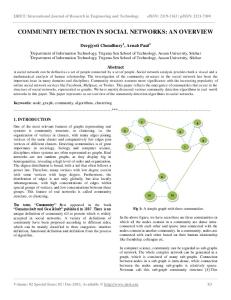
Chapter 3: Methodology The methodology consisted of three major phases. In the first phase, articles and comments posted on them were collected (Section 3.1) and annotated (Section 3.1.1, page 17) to create an annotated corpus. Pre-processing was also performed to remove URLs and stop words from the data. In the second phase (Section 3.2, page 19) a machine learning model was developed to detect controversial trends, including identification, calculation, analysis, and extraction of features including sentiment and controversy scores. The third phase was analysis and improvement of performance of the model, discussed in Chapter 4, page 21. 3.1 Data Collection This research involved development of a new controversy corpus. The corpus consists of comments made by viewers on 728 articles published by Cable News Network (CNN) on its online news portal1. CNN is a broadcast news company based in the U.S. offering world news on its cable T.V. channel as well as on its website. CNN.com utilizes the Disqus Plugin to permit readers to post comment and provide feedback on their news stories. Disqus is an online discussion and commenting service provider for websites. It allows users to comment by logging in using their existing accounts with other social media websites (i.e. Twitter, Facebook, Google+, etc.) without having to create a new user account (Disqus, 2012). To collect data, an application was created using VB.NET. A screenshot of the application is shown in Figure 1. The application collected a list of news articles posted on CNN.com using Disqus API2. Using the list of news articles, CNN.com was crawled to gather the articles’ text. Comments posted on the articles and information about the users who commented was collected by making calls to the Disqus API. The comments were accessed for an article via the Disqus API using http://disqus.com/api/3.0/threads/listPosts.json?api_key=[api_key]&forum=cnn&limit=100&thre ad=link:[article_url]. Disqus API works over the HTTP protocol as a REST web service. When a GET request is sent, the API returns data in JSON format. There is a limit of 1000 request per day with each request containing a maximum of 100 objects. In the returned JSON a cursor is provided for the next set of posts. An example of comments data returned for the article titled “Rescuers search for missing after deadly Hong Kong ferry crash” is displayed in Figure 2. Data elements returned by the Disqus API are displayed in Table 1. All information retrieved was stored in an SQL database. The Entity Relationship Diagram (ERD) of the database is displayed in Figure 3.

1 2

http://cnn.com http://disqus.com/api/docs/

13

Figure 1: Data collection

Figure 2: Example of comments returned by the Disqus API

14

article PK

annotation

id

int

PK

annotationID int identity

title createdAt link category

varchar(255) datetime text int

FK1 FK2

articleID userid controversial

users

comments PK

FK1

FK2

int int bit

id

int

parentCommentId comment threadId createdAt likes userid posScore negScore

int text int datetime int int smallint smallint

PK

userID

int identity

username email pwd

varchar(255) varchar(150) varchar(100)

cnn_users PK

id

int

username about name ProfileURL joinedAt reputation

varchar(100) text varchar(150) varchar(255) datetime float

Figure 3: Database ERD Table 1: Data elements returned by the Disqus API Author username

user name of the author

id

user id of the author

name

name of the author

about

text about the author

url

URL to the author’s profile page

reputation

reputation score of the author

Comment message

comment text

id

id of the comment

parent

id of the original comment if the comment is a reply to another comment

likes

number of likes

15

3.1.1 Annotation To aid in annotation, a web application was created. Each article was annotated by at least 3 annotators. There were a total of 20 annotator from various educational backgrounds – 2 from business, 2 from education, 3 from engineering, 6 from humanities, 3 from sciences, 4 from social sciences. The annotators were given the definition of controversy (see Figure 4) and were instructed to identify which articles they think are controversial. The annotators were displayed articles along with their respective comments (see Figure 5). For each article, the annotators classified whether the article is controversial or not. When there was a conflict between annotators in classifying an article, then a voting scheme was be used where the class with the majority votes won. Inter-annotator agreement statistics are discussed in Chapter 4, page 19.

Figure 4: Definition of controversy The annotations were stored in the "annotation" table with the userid of the annotator, articleID of the article being annotated, and classification made by the annotator as shown in Figure 3. When the annotator classified an article as controversial then 1 was stored in the "controversial" column, otherwise a 0 was stored. An Institutional Review Board (IRB) exemption from institutional oversight was obtained (see Appendix B, page 44).

16

Figure 5: Example of the annotation process 3.1.2 Preprocessing After the data was collected, URLs from the comments were removed. Some articles containing only an image gallery were removed since there was no textual information in the article. A total of 72 articles were removed from the original 800 collected bringing the total number of articles in the corpus to 728. Since stop words do not provide any information and introduce noise, they were removed using a stop word list. The preprocessing application was developed in the windows environment in VB.NET.

17

3.2 Controversy Trend Detection To detect which articles are controversial, the sentiment of the comment text was analyzed using SentiStrength (Thelwall et al., 2012) to classify whether the viewer is expressing positive, negative, or neutral. After the sentiment classification was done, a controversy score was calculated and other features - number of posts, post rate, number of posts with positive sentiment, number of posts with negative sentiment, number of ‘Likes’, number of posts with responses from other viewers, controversy term count in article text, sum of controversy term count in comments text, average comment word count, sum of user reputation score, total number of users, total number of new users since article post were extracted. The controversy score was calculated by dividing total number of negative comments the ratio of negative sentiment count to positive sentiment count. Pseudocode for calculating the controversy score and the post rate of an article is shown in Figure 6. The presence of controversy terms in comments and articles’ texts were done by creating a controversy term list from “Wikipedia: List of controversial issues”3. To predict how soon a controversial article can be detected, the comments for their respective articles were divided into time spans of 6hr, 12hr, 18hr, 24hr, 30hr, 36hr, 42hr and 48hr. For each of the time spans, features were extracted and a Decision Table classifier was trained and tested to see how well the classifier performs using the features extracted from comments belonging to a specific time interval. All the features were normalized between 0 and 1. Features used for this research are listed below with features unique to this research marked with an asterisk:           

3

Comment count(t) – total number of comments by time t Comment post rate(t) – post rate of comments per hour by time t Likes(t)* – number of ‘Likes’ by time t Threaded comments count(t)* – number of comments which have responses from other users by time t Positive sentiment count(t) *– total number of positive comments by time t Negative sentiment count(t)* – total number of negative comments by time t Controversy score(t)* – negative sentiment comment count divided by sum of positive sentiment comments count and negative sentiment comments count by time t Reputation(t)* - aggregate reputation scores of users who posted on an article by time t Number of users(t)* - total number of users who commented on an article by time t New users(t)* - total number of new users who commented on an article by time t Article controversy term count* - number of controversy terms that appear in the article text

http://en.wikipedia.org/wiki/Wikipedia:List_of_controversial_issues

18

 

Comment controversy term count(t)* - total number of controversy terms that appear in all the comments posted on an article by time t Word count(t)* - average word count of comments posted on an article by time t

The sentiment scores for comments were calculated using an application called SentiStrength, which estimates the strength of positive and negative sentiment in short texts. SentiStrength reports two sentiment strength: -1 (not negative) to -5 (extremely negative) and 1 (not positive) to 5 (extremely positive) (Thelwall et al., 2012). The sentiment strength scores returned by SentiStrength were stored in the comments table as shown in Figure 3, page 16.

Figure 6: Pseudocode for calculating controversy score and post rate

19

Chapter 4: Results and Analysis To predict how soon an article can be detected as being controversial or not, the data was divided into 6 hour time spans - 6hr, 12hr, 18hr, 24hr, 30hr, 36hr, 42hr and 48hr. For each time span features were extracted from comments posted within the time interval (e.g. in 6hr time span, features were extracted from comments posted within the first six hours of the article being posted). From the controversy corpus containing 728 articles, 664 articles were chosen since 64 articles did not have any comments in the first six hours of the article being posted. Each of the time spans contained features for 664 articles, of which 365 articles were controversial and 299 were non-controversial. Decision Table classifier was used for training and testing. Ten-fold cross validation was used to minimize the impact of specific case selection on performance results. Performance as a function of time span was measured. F-Measure was used to measure the performance of the methodology. Formulae for F-score calculation is displayed in Figure 7.

Figure 7: F-Score calculation 4.1 Controversy Corpus To measure the quality of the annotation process, inter-annotator agreement Kappa ( ) was calculated. The calculation is based on the difference between how much agreement among annotators is actually present compared to how much agreement would be expected to be present by chance alone. The formula for calculating is shown below.

𝜅=

𝑃 − 𝑃𝑒 1 − 𝑃𝑒

𝑃 denotes the mean value of 𝑃𝑖 ’s, where 1 ≤ 𝑖 ≤ 𝑁, is the extent to which annotators agree for the 𝑖 𝑡ℎ classification. Whereas 𝑃𝑒 denotes the sum of squares of 𝑝𝑗’s, where 1 ≤ 𝑗 ≤ 𝑘, is the proportion of all the assignments which were to the 𝑖 𝑡ℎ sample. Therefore, 𝑃 − 𝑃𝑒 gives the

20

degree of agreement actually present and 1 − 𝑃𝑒 gives the degree of agreement that is attainable above chance. A value of 0.33 was obtained. The value of was compared with the interpretation of Kappa first studied by Landis and Koch (1977) as shown in Table 2. The obtained value of can be interpreted as fair agreement between annotators. Table 2: Interpretation of Kappa Interpretation