CONSTRAINED OPTIMIZATION OF MULTILAYERED ANTI-REFLECTION COATINGS USING GENETIC ALGORITHMS Kai-Yew Lum 1∗, Pierre-Marie Jacquart 2 and Mourad Sefrioui 2 1

Temasek Laboratories, National University of Singapore, 10 Kent Ridge Crescent, Singapore 119260 2 Dassault Aviation, 78 Quai Marcel Dassault – Cedex 300, 92552 St Cloud Cedex, France

Abstract– Optimization based on genetic algorithms is applied to the design of multilayered coatings, incorporating both coating-geometry and material-property optimization. The latter is based on parametric modeling of dielectric and magnetic properties of homogeneous materials, and effective-medium modeling of composites. Our approach treats physical laws to be obeyed by the models as constraints. Moreover, efficiency in thickness is considered in two ways: as a constraint on its upper limit, and in a multi-objective setting where we study both aggregation and Pareto optimality. 1. INTRODUCTION Anti-reflection coatings are widely used for optical and highfrequency applications such as dichroic filters in optics, or microwave absorbing materials for electromagnetic compatibility. Even though a single-layer coating may be sufficient to obtain low reflection coefficients, its efficiency is usually reduced to a narrow bandwidth and to a specific polarization and incidence angle. In such a case, analytical expressions can be obtained [1, 2], even for strongly anisotropic mediums [9], to define the criteria (refractive index, dielectric permittivity, magnetic permeability) that a monolayer has to satisfy in order to achieve the desired antireflection properties. Nevertheless, these criteria are usually approximate close-form expressions that are based on certain hypotheses. In order to extend the performance of anti-reflection coatings to wider ranges of frequency and incidence, a multilayered structure has to be considered. The problem of optimal design of a multilayered coating has been studied in the past using analytical – the conjugate gradient – and stochastic methods such as simulated annealing (see [11] and references therein). Thus, the optimization of such complex architectures may consist either in optimizing the thickness of well-defined materials chosen from a database in a purely combinatorial problem [11], or in determining parameters involved in functional descriptions of the main properties of materials. ∗ Research

partially funded by the French Government.

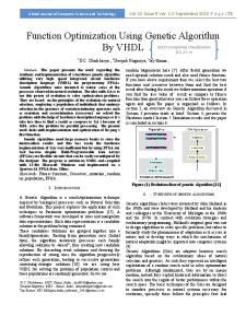
In this study, we focus on the optimal design of the material properties themselves, in addition to the geometry of the coating (thickness for a 1D problem). We also consider heterogeneous layers in order to achieve performance that may not be easily obtained with homogeneous layers. Thus, the optimization of such complex multilayered coatings now entails the determination of many parameters (e.g. we shall consider a problem with 21 unknowns) that may not be easily solved in an analytical approach. As the models describing each material or composite are complex parametric functions of frequency, constraints are imposed to ensure that the materials obtained have physical significance. The present approach fits into the class of of constrained multivariable, multi-objective design problems to which GA has demonstrated remarkable applicability, e.g. [3, 10]. In particular, we adopt binary coding which allows the control of the search space to correspond to realistic manufacturability. Moreover, we study multi-objective problems using the technique of Pareto optimality, which yields a selection of designs of equal merits vis-a-vis the trade-off between reflectivity and thickness. 2. PROBLEM DESCRIPTION Consider the multilayered coating shown in Figure 1 which consists of M layers of different materials covering a perfectly electrical conductor at the base. For our purpose, the material in the k-th layer is characterized by its dielectric and magnetic properties, as well as its thickness, i.e. by



θ 



                                   µ M )        Layer M M,             (ε  













































  























 
 

  

  
  

  

  
  Layer  

  1
  

  

  (ε
  1
, 
 µ
1)      PEC                             Figure 1. Multilayered Coating

hM

h1

the triplet (
k , µk , hk ) for k ∈ {1, ..., M }. In all that follows, we shall adopt the e2πf t convention to describe the propagation of an electromagnetic wave incident on a material. Then, for homogeneous materials that either constitute a monolayer or inclusions embedded in a host, the permittivity and permeability can be written as functions of the frequency f :
k (f ) =

k (f ) − 


k (f ) b
bk + ck f ) − (a
k + k + c
k f ), f f µk (f ) = µ
k (f ) − µ

k (f ) = (ak +

= αk +

βk + βk
f . γk − f 2 + γk
f

(1)

(2)

where

k ,...,µ

k are real-valued functions, and ak ,...,c
k and αk ,...,γk
are real coefficients, Equation (2) is known as the Lorentz formula. The combination of (1) and (2) models a wide range of materials that includes lossless and lossy dielectric and magnetic materials [6]. For composite materials,we consider models proposed by various effective medium theories, such as the Bruggeman and the Maxwell-Garnett models. For example, in the Bruggeman model, if the material in layer k is composed of spherical inclusions A with electrical resistivity ρk and radius rk , embedded in a host B with filling factor φk , then it has the effective permeability µk governed by the following equation which depends on the parameters (rk , ρk , φk ) [4, 13, 14]: µA (f, rk , ρk ) − µk (f ) µB (f ) − µk (f ) +(1−φk ) = 0. µA (f, rk , ρk ) + 2µk (f ) µB (f ) + 2µk (f ) (3) With the above description, the problem becomes one of parametric design. Let the various parameters defining permittivity, permeability and thickness be collectively denoted vi , for i = 1, ..., n where n is the total number of parameters. The design objective consists in manipulating the vi ’s such that the coating exhibits low refl ection. Let then the refl ectivity cost function be defined by the average of refl ection coefficients R(fp , θq ) over a discrete range of frequencies fp (p = 1, ..., Nf ) and incident angles θq (q = 1, ..., Nθ ):

impose on the design a maximum allowable total thickness. In Section 4, we further explore the multiple-objective problem where one desires to obtain minimum refl ection with minimum coating thickness. We employ for the present problem a basic form of genetic algorithms, i.e. with fixed-size populations, gray binary coding, and crossover and mutation operators for binary strings (see Figure 2). In addition, the selection operator is based on the principle of stochastic tournament with replacement. The reader may refer to [5, 7], for example, for descriptions of such an algorithm and comparisons with other variants. In the following, we shall discuss in more details the formulation of objective functions and constraint penalties for the particular problem we are studying. Note also that we work in the minimization setting, i.e. a fitter solution has a lower fitness value. Initial Population P0

i

i+ 1

Decode Pi Calculate Fitness & Penalty

Select Pair Crossover

Filled P ? i+1

No

φk

Nf Nθ
1
 R(v1 , ..., vn ) = R(fp , θq ). Nf Nθ q=1 p=1

(4)

R takes values between 0 and 1. The optimal coating is therefore one that minimizes R over an admissible set A of parameters: R∗ = min R(v1 , ..., vn ). (5) A

In addition, the design may be subject to a penalty on the extra weight contributed by the coating. This may be accounted for through two basic approaches: in Section 3 we

Mutate Pi+1 Check Stop ?

Continue

Stop

Figure 2. Flowchart of Genetic Algorithm with Penalty on Constraint Violation

3. SINGLE-OBJECTIVE OPTIMIZATION For single-objective optimization of the coating, the fitness function of a design equals the cost function R(v1 , ..., vn ) penalized by the constraint-handling process described below. A design is considered non-feasible if it contains nonphysical materials or if its total thickness exceeds the allowed maximum. Handling constraints by penalizing instead of simply eliminating the non-feasible designs has the advantage of allowing the latter to participate in the evolution process, thus keeping a genetically diverse population while favoring feasible designs.

3.1. Constraint on physical admissibility The parametric representation of materials proposed in Section 2 entails a question on its physical admissibility. Indeed, in order for a representation to comply with the physical law of dissipation, the imaginary parts


k and µ

k must be positive for all frequencies. For the Lorentz formula (2) this condition corresponds to some algebraic constraints on the parameters. Moreover, as (2) is an abstract form of Gilbert’s frequency response model [6], the coefficients in (2) are not mutually independent. For composite materials, the admissibility condition becomes even more complex. Instead of dealing with the algebraic constraints on the parameters whose forms depend eventually on the permeability function, we choose to simply compute the imaginary part µ

k (f ) over the frequency range of interest, and define the following penalty function for the k-th layer:   if µ

k (f ) ≥ 0 ∀f,   0  Nf
Ck =


(6)  |µ

k (fi )| otherwise. |µk (fi− )|   i=1

i−

−

where i are the indices for which µ

k (fi− ) are negative. Note that Ck equals 0 for physically admissible materials, and takes positive values up to 1 for non-physical materials. Then the total penalty on the coating is simply the sum: C=

M


Ck .

(7)

k=1

This approach is obviously independent of the modeling function used. 3.2. Constraint on total thickness M Let the total thickness be denoted by H = k=1 hk on which one imposes an upper limit Hmax . The corresponding penalty function on a design is defined as  0 if H < Hmax , D= (8) H/Hmax − 1 otherwise.

Algorithm 1. Let J + denote the maximum value of the cost function (9) among the feasible solutions, and J − the minimum among the non-feasible ones. Then, the SFP fitness is given by F = R + pc C + pd D + δSFP , (10)

δSFP =



0 if solution is feasible, max(J + − J − , 0) otherwise.

(11)

Moreover, if all solutions are feasible or if all solutions are non-feasible, δSFP is zero for all solutions, i.e. no adjustment is needed. 4. MULTIPLE-OBJECTIVE OPTIMIZATION In this section we shall further consider the problem of multiple objectives. Indeed, here we seek a design that produces minimum refl ection with minimum thickness. This consideration is reasonable from a practical and economical viewpoint. However, from a physical viewpoint, such a solution may not exist. Indeed, for relaxation-type dielectric or magnetic materials, thicker coatings means lower refl ection [8]. So, in general, the two objectives are incompatible. Note also that treating thickness as an objective function does not exclude imposing on it an upper limit at the same time. 4.1. Aggregate Cost Function A straight-forward approach to multiple objectives consists in aggregating the two cost functions by a linear combination; thus, the SFP fitness function as given in (10) now becomes: FSFP = λr R + λh H + pc C + pd D + δSFP ,

(12)

D is therefore the fraction of Hmax by which a design violates the thickness constraint.

where λr and λh are weights to be chosen, and δSFP is calculating as defined in Algorithm 1. Optimization then proceeds in exactly the same manner as for the single-objective problem. This approach is similar to that in [11]. It is wellknown that the solution produced by aggregation is sensitive to the choice of the weights λr and λh . In particular, choosing the coefficients requires a priori knowledge of the relative orders of magnitude of R and H (see Section 5.1).

3.3. Superiority of feasible points (SFP)

4.2. Pareto Optimality

The penalty functions C and D are used to penalize the fitness of a design. First, consider the following penalized cost function: J = R + pc C + pd D, (9)

Instead of aggregation, we also consider multi-objective optimality in the sense of Pareto [3, 5, 7]. We may in the first place consider the fitness of a design be defined as its Pareto rank. Note that in our context of minimization, rank zero corresponds to non-dominated designs, and higher ranks are assigned to successive Pareto fronts. Now, in order to extend the notion of superiority of feasible points to the current setting, we adopt the principle that a feasible solution

where pc and pd are constant penalty coefficients to be chosen. However, the above does not guarantee that a feasible solution has a better (smaller) fitness than a non-feasible one. To do so, we adopt a basic SFP approach [12]:

necessarily dominates a non-feasible one. This yields the following modified SFP algorithm: Algorithm 2. Let the cost functions: J1 = R + pc C + pd D, J2 = H + pc C + pd D.

(13) (14)

Using the same notation as in Algorithm 1, consider the following SFP adjustments in the general case (the special cases where all designs are feasible or all are non-feasible need no adjustment):  0 if solution is feasible, δi = (15) max(Ji+ − Ji− , 0) otherwise; with i ∈ {1, 2}. Then, the multi-objective SFP cost functions to be used in the Pareto ranking process are simply given by Fi = Ji + max(δ1 , δ2 ),

i ∈ {1, 2}.

(16)

Let ρ denote the Pareto rank of a design. Simple rankbased fitness assignment may lead to genetic drift, i.e. the populations tend to converge to a localized point on the global Pareto front instead of spanning the whole front. To prevent this, we adopt the fitness sharing approach based on the principle that similar designs (according to the Hamming distance) mutually decrease each other’s fitness by competing for the same resources. Isolated solutions are thus given a greater chance of reproducing [3, 7]. The resulting shared fitness of a design has S the form: Fshared (S) = ρ(S) + σ(S),

5.1. Single-Objective Examples In this section, we consider two examples where the fitness function is the refl ectivity function (4). Example 1 consists of a two-layers of homogeneous, lossy dielectrics with permittivities described by (18). The thickness of each layer is fixed at 5 mm. A population size of 20 is chosen. As shown in Figure 3, convergence is achieved after about 700 iterations, i.e. 35 generations. The spectral refl ection coefficient is shown in Figure 5, where one can see that 15 dB attenuation or better is achieved mainly in the 8-16 GHz range. Example 2 is a two-layer structure of composite materials with a maximum total thickness of 5 mm. Each layer is composed of lossy dielectric and magnetic inclusions with properties described by (2) and (18), embedded in a lossless host. The macroscopic properties of each composite are approximated by the Bruggeman model (3). The population size is 100, and the refl ectivity converges to -14.7 dB in 100 generations, as shown in Figures 4. The final design is summarized in the following table. Example 2: Final design of 2-layer composites Substrate:
= 1.45, µ = 1.0. Layer 1 inclusion properties, composition and thickness: 1995.7+0.319
1 = 3.02 −  320.0 µ1 = 1 + 197.2− 2 +0.449 , f , r1 = 1µm, ρ1 = 185, φ1 = 22.5%, h1 = 1.43 mm. Layer 2 inclusion properties, composition and thickness: 1920.3+0.273
2 = 3.35 −  1730.0 , µ2 = 1 + 0.0− 2 +0.061 , f r2 = 3µm, ρ2 = 197.5, φ2 = 30.0%, h2 = 3.57 mm.

(17)

where the sharing function σ takes values in [0, 1). The effect of sharing on a design is that its Pareto rank is deteriorated (augmented) by as much as it is genetically “crowded”. However, a solution is never “demoted” to the next rank as the augmentation is always less than 1.

This example demonstrates the ability of the approach to handle complex structures. Compared to the dielectric design in Example 1, the composite structure in Example 2 yields lower refl ectivity despite having only half the total thickness (see Figure5). Better than 15 dB attenuation is achieved over a wider range of 4-16 GHz.

5. NUMERICAL RESULTS 5.2. Multi-Objective Example We present here two single-objective examples, and a third on multi-objective optimization where we shall compare the aggregate and Pareto approaches. The refl ection coefficients are computed at normal incidence and over the frequency range 1–20 GHz using a Maxwell equation solver. In the following, let Np denote the population size1 . Without loss of generality, we shall consider in the examples that follow a simplified form of the permittivity function (1): b

k (f ) = ak −  k . f

(18)

1 These examples should meanwhile be treated as numerical demonstrations of the proposed approach; whether the resulting designs can be practically fabricated remains to be studied.

Here, we consider a two-layer structure of magnetic materials, each described by the lossy dielectric and magnetic model given by (2) and (18). Three cases are considered: Case A: Single objective, where the fitness equals the refl ectivity function (4). Population size equals 100. Case B: Linear combination of refl ectivity and thickness through the aggregate fitness function (12), with λr =1, λh =10−6 . Population size equals 100. Case C: Multi-objective Pareto optimality. Here, population size equals 400.

The penalty coefficients used in Algorithm 1 or Algorithm 2, depending on the cases, are pc = 1 and pd = 0.5. As shown in Figures 6 and 7, Case A produces a lower refl ectivity than Case B (R∗A = −77.7 dB, R∗B = −65.5 dB), ∗ while Case B produces a thinner structure (HA = 2.1 + ∗ 4.1 mm, HB = 1.3 + 3.2 mm). This is due to the fact that in Case B, as R descends below -60 dB which equals the weight λh , the thickness becomes dominant in the aggregate cost function. As a result, the aggregate method seeks a thinner structure instead of one with lower refl ectivity. This shows that the approach is sensitive to the choice of weights. The spectral behavior of the final designs for Cases A and B are compared with those of Examples 1 and 2, where one can see that much better broad-band attenuation is achieved by optimizing two homogeneous magnetic layers as in the present example. Finally, Figure 8 shows the points forming the Pareto fronts of successive generations, which reveal a part of the global Pareto front after 20,000 iterations. This result is not entirely satisfactory as the Pareto front does not either include or dominate the final solutions of Cases A and B as one would expect. The populations have a tendency to converge toward the upper part of the front, in spite of fitness sharing.[10] Nevertheless, the advantage of Pareto ranking is evident in its ability to reveal a set of designs of equal merit. For example, some of these yield -35 dB with a thickness of only 1 mm, a result that would have been difficult to obtain with the single-objective or aggregate methods. 6. DISCUSSION & CONCLUSION For single and aggregate objective problems, the optimization algorithm in this paper is similar to that employed in, say, [11]. However, the two approaches differ in material modeling where the cite reference employed a combination of known materials while presently, we are optimizing unknown materials. Comparing the results of Example 2 and Cases A and B of Example 3, with the broad-band results BB1 and BB2 in [11], one can say that similar or better broad-band results can be achieved in the present approach with two-layer structures, whereas [11] required five layers, although the net thicknesses are comparable. With recent advances in composites where one may obtain desired permittivity and permeability functions by manipulation parameters such as fill factor and grain size, we believe the present approach offers an useful tool for determining the target designs in material synthesis. Nevertheless, the multi-objective problem is particularly difficult, where simple fitness sharing is not sufficient to explore the global Pareto front. One may consider the selection sharing method in [10]. However, the front is genetically diverse and may require additional mechanisms to explore.

The present work is limited to one-dimensional optics. Future work consists in extending to quasi two dimensions where incidence angles are more realistically determined by the shape. Moreover, it will be interesting to apply more sophisticated techniques such as parallelization and hierarchical algorithms in order to alleviate the heavy computation loads in 2D design [15]. 7. REFERENCES [1] R.M.A. Azzam and N.M. Bashara. Ellipsometry and Polarized Light. North-Holland, Amsterdam, 1997. [2] M. Born and E. Wolf. Principles of Optics. Pergamon Press, 1st edition, 1959. [3] M.-O. Bristeau, R. Glowinski, B. Mantel, J. P´eriaux, and M. Sefrioui. Genetic algorithms for electromagnetic backscattering: Multiple objective optimization. In E. Michielssen and Y. Rahmat-Samii, editors, Electromagnetic Optimization by Genetic Algorithms. J. Wiley, New York, 1999. [4] D.A.G. Bruggeman. Berechnung verschiedener physikalischer konstanten von heterogenen substanzen. Ann. Physik. (Leipzig), 24:636–679, 1935. [5] D.A. Coley. An Introduction to Genetic Algorithms for Scientists and Engineers. World Scientific, Singapore, 1999. [6] T.L. Gilbert. A Lagrangian formulation of gyromagnetic equation of the magnetization field. Physical Review, 100(4):1243, 1955. [7] E.D. Goldberg. Genetic Algorithms in Search, Optimization and Machine Learing. Addison-Wesley, Reading, MA, 1989. [8] P. Hartemann and M. Labeyrie. Absorbants d’ondes e´ lectroniques. Revue Technique Thomson-CSF, 19:413, 1987. [9] Pierre-Marie Jacquart, O. Acher, and P. Gadenne. Refl ection and transmission of an electromagnetic wave in a strongly anisotropic medium: application to polarizers and antirefl ection layers on a conductive plane. Opt. Comm., 108:355, 1994. [10] R.A.E. Makinen, J. Periaux, and J. Toivanen. Multidisciplinary shape optimization in aerodynamics and electromagnetics using genetic algorithms. International Journal for Numerical Methods in Fluids, 30:149–159, 1999.

[11] E. Michielssen, J.-M. Sajer, S. Ranjithan, and R. Mittra. Design of lightweight, broad-band microwave absorbers using genetic algorithms. IEEE Trans. on Microwave Theory & Techniques, 41:1024–1030, 1993. [12] K. Miettinen, M.M. Makela, and J. Makinen. Handling constraints with penalty techniques in genetic algorithms – a numerical comparison. Number B 10/1999 in Reports of the Dept. of Mathematical Information Technology. University of Jyvaskyla, 1999.

20 Example 1 : Dieletrics (10mm) Example 2 : Composites (5mm) Example 3A: Magnetics (6.2mm) Example 3B: Magnetics (4.5mm)

0 -20 -40 -60 -80 0

[13] G.A. Niklasson, C.G. Granqvist, and O. Hunderi. Effective medium models for the optical properties of inhomogenious materials. Applied Optics, 20(1):26–30, Jan. 1981.

[15] M. Sefrioui and J. P´ eriaux. A hierarchical genetic algorithm using multiple models for optimization. In 6th International Conference in Parallel Problem Solving from Nature – PPSN VI, LNCS 1917, Paris, France, September 2000. Springer.

4

6

8 10 12 Frequency (GHz)

14

16

18

20

90

100

Figure 5. Refl ection coefficients 0 Case A Case B

-10

Reflectivity (dB)

[14] D. Rousselle, A. Berthault, O. Acher, J.P. Bouchard, and P.G. Z´ erah. Effective medium at finite frequency: Theory and experiment. Journal of Applied Physics, 74:475, 1993.

2

-20 -30 -40 -50 -60 -70 -80 0

10

20

30 40 50 60 70 No. of iterations (x100)

80

Figure 6. Evolution of Refl ectivities (Cases A & B) -3 Min. Reflectivity Mean Reflectivity Historical Mean

10

-5

Case A Case B

8

Thickness (mm)

Reflectivity (dB)

-4

-6 -7 -8 -9

6 4 2

-10 0

100

200

300 400 No. of iterations

500

600

700

0 0

10

20

30

40

50

60

70

80

90

100

No. of iterations (x100)

Figure 3. Two-layer dielectric structure (Example 1) Figure 7. Evolution of total thickness (Cases A & B) 0

Reflectivity (dB)

-4

Reflectivity (dB)

Min. Reflectivity Mean Reflectivity Historical Mean

-2

-6 -8 -10 -12 -14 -16 0

20

40 60 No. of iterations (x100)

80

Figure 4. Two-layer composite structure (Example 2)

100

0 -10 -20 -30 -40 -50 -60 -70 -80 0.01

Pareto front Case B Case A 0.1

1 Thickness (mm)

Figure 8. Pareto Front (Case C)

10