Computing Best Coverage Path in the Presence of Obstacles in a Sensor Field Senjuti Basu Roy, Gautam Das, and Sajal Das Department of Computer Sc and Engineering. University of Texas At Arlington, Arlington, TX-76019 {roy,gdas,das}@cse.uta.edu
Abstract. We study the presence of obstacles in computing BCP (s, t) (Best Coverage Path between two points s and t) in a 2D field under surveillance by sensors. Consider a set of m line segment obstacles and n point sensors on the plane. For any path between s to t, p is the least protected point along the path such that the Euclidean distance between p and its closest sensor is maximum. This distance (the path’s cover value) is minimum for a BCP (s, t). We present two algorithmic results. For opaque obstacles, i.e., which obstruct paths and block sensing capabilities of sensors, computation of BCP (s, t) takes O((m2 n2 + n4 ) log(mn + n2 )) time and O(m2 n2 + n4 ) space. For transparent obstacles, i.e., which only obstruct paths, but allows sensing, computation of BCP (s, t) takes O(nm2 + n3 ) time and O(m2 + n2 ) space. We believe, this is one of the first efforts to study the presence of obstacles in coverage problems in sensor networks.
1
Introduction
In this paper, we study a specific class of problems that arises in sensor networks, and propose novel solutions based on techniques from computational geometry. Given a 2D field with obstacles under surveillance by a set of sensors, we are required to compute a Best Coverage Path (BCP ) between two given points that avoids the obstacles. Informally, such a path should stay as close as possible to the sensors, so that an agent following that path would be most “protected” by the sensors. This problem is also related to the classical art gallery and illumination research type of problems that has been long studied in computational geometry [14,15]. However, there are significant differences between the problem we consider and these other works, which we elaborate later in the paper. Moreover, to the best of our knowledge, ours is one of the first efforts to study the presence of obstacles in coverage problems in sensor networks. More formally, let S = {S1 , . . . , Sn } be a set of n homogeneous wireless point sensors deployed in a 2D sensor field Ω. Each sensor node has the capability to sense data (such as temperature, light, pressure and so on) in its vicinity (defined by its sensing radius). For the purpose of this paper, assume that these sensors are guards that can protect any object within their sensing radius, except F. Dehne, J.-R. Sack, and N. Zeh (Eds.): WADS 2007, LNCS 4619, pp. 577–588, 2007. c Springer-Verlag Berlin Heidelberg 2007 �
578
S.B. Roy, G. Das, and S. Das
that the level of protection decreases as the distance between the sensor and the object increases. Let P (s, t) be any path between a given source point s and a destination point t. The least protected point p along P (s, t) is that point such that the Euclidean distance between p and its closest sensor Si is maximum. This distance between p and Si is known as the cover value of the path P (s, t). A Best Coverage Path between s and t, BCP (s, t), is a path that has the minimum cover value. A BCP is also known as a maximal support path (MSP). In recent years there have been several efforts to design efficient algorithms to compute them [5,9,10]. However, one notable limitation of these works is that they have not considered the presence of obstacles in the sensor field, i.e., objects that obstruct paths and/or block the line of sight of sensors. In fact, most papers that deal with coverage problems in sensor networks have not attempted to consider the presence of obstacles. This is surprising since obstacles are especially realistic in a deployment of sensors in unmanned terrain (e.g., buildings and trees, uneven surfaces and elevations in hilly terrains, and so on). In this paper we study the presence of obstacles in computing best coverage paths. However we do not consider the length of the path (i.e., minimizing the path length) in the computation of a BCP . More formally, assume that in addition to the n sensors, there are also m line segment obstacles O = {O1 , . . . , Om } placed in the sensor field. Line segments are fundamental building blocks for obstacles, as more complex obstacles (e.g., polygonal obstacles) can be modeled via compositions of line segments. We consider two types of obstacles: (a) opaque obstacles which obstruct paths as well as block the line of sight of sensors, and (b) transparent obstacles which obstruct paths, but allow sensors to “see” through them. Examples of the former may include buildings - they force agents to take detours around them as well as prevent certain types of sensors (such as cameras) from seeing through them - while examples of the latter may include lakes - agents only have to take detours around them but cameras can see across to the other side. When obstacles are opaque, we refer to the best coverage path problem as the BCP (s, t) Problem for Opaque Obstacles, whereas for transparent obstacles, we refer to the problem as the BCP (s, t) Problem for Transparent Obstacles. Figure 1 is an example of a BCP (s, t) amidst two sensors and four opaque obstacles, whereas Figure 2 shows a BCP (s, t) in the same sensor field but assumes the obstacles are transparent.1 To compute BCP (s, t) without obstacles, existing approaches [5,9,10] leverage the fact that the Delaunay triangulation of the set of sensors - i.e., the dual of the Voronoi diagram - contains BCP (s, t). Furthermore, [9] shows that sparse subgraphs of the Delaunay triangulation, such as Gabriel Graphs and even Relative Neighborhood Graphs contain BCP (s, t). However, such methods do not easily extend to the case of obstacles. Moreover, as should be clear from Figure 1, the visibility graph [2] is also not applicable to the BCP (s, t) problem for opaque 1
We assume infinite sensing capabilities for our sensors; although sensing intensity decreases with the increased distance. Generalizing our algorithms for a finite sensing radius is straightforward and omitted from this paper.
Computing Best Coverage Path in the Presence of Obstacles
579
s O1 s
Bisector between two point S1 and S2
cover
S1
p (least protected point)
S1 O1
O2 cover p (least protected point)
O2
O3 S2
O3
S2
t
O4
t O4
Fig. 1. A BCP (s, t) for Opaque Obstacles
Fig. 2. A BCP (s, t) for Transparent Obstacles
obstacles, as the best coverage paths in this case need not follow edges of the visibility graph. In fact, to solve the BCP (s, t) problem for opaque obstacles, we have developed an algorithm that takes quartic-time, based on constructing a specialized dual of the Constrained and Weighted Voronoi Diagram (henceforth known as the CW-Voronoi diagram) [13] of a set of point sites in the presence of obstacles. This type of Voronoi diagram is a generalization of Peeper’s Voronoi Diagram [6] that involves only two obstacles. These two Voronoi diagrams are different from other Voronoi diagrams involving obstacles studied in papers such as [3,1,11] - since the latter requires that every obstacle endpoint be a site whereas in the former the Voronoi sites are distinct from the obstacle endpoints. Unlike standard Voronoi diagrams for point sets without obstacles, the Voronoi regions in a Peeper’s Voronoi diagram site may be disconnected [6]. However, for the BCP (s, t) problem with transparent obstacles, we have shown that a best coverage path is contained in the visibility graph (with suitably defined edge weights), which enables us to develop a more efficient algorithm for it. As mentioned earlier, the BCP (s, t) problems are also related to art gallery problems [14,15], which are concerned with the placement of guards in regions to monitor certain objects in the presence of obstacles. An early result in art gallery research, due to V. Chv´ atal, asserts that � n3 � guards are occasionally necessary and always sufficient to guard an art gallery represented by a simple polygon of n vertices [14,15]. Since then, numerous variations of the art gallery problems have been studied, including mobile guards, guards with limited visibility or mobility, guarding of rectilinear polygon and so on. The main difference between the the art gallery problems and the BCP problems is that the former problems (such as Watchman Route, Robber Route [14,15] and so on) attempt to determine paths that minimize total Euclidean distances under certain constraints, whereas the metric to be minimized in the latter problems (the cover of the path) is sufficiently different from Euclidean distance, thus requiring different approaches.2 A comprehensive survey of art gallery research is presented in [15]. 2
It is easy to prove that the cover is a metric, and holds all metric properties. We omit the proof from this version of the paper.
580
S.B. Roy, G. Das, and S. Das
In this work, our contributions may be summarized as follows: – We have initiated a study of the presence of obstacles and their impact in the computation of BCP. We have shown that obstacles significantly complicate BCP computations. We have developed two variants of the problem, the BCP (s, t) problem for opaque obstacles and the BCP (s, t) problem for transparent obstacles, based on variants of obstacle properties. – We have designed an O((m2 n2 + n4 ) log(mn + n2 )) time and O(m2 n2 + n4 ) space algorithm for computing BCP (s, t), given n sensor nodes and m opaque line obstacles. – We have designed an O(nm2 + n3 ) time and O(m2 + n2 ) space algorithm for computing BCP (s, t), given n sensor nodes and m transparent line obstacles. The rest of the paper is organized as follows: In Section 2 we describe our algorithm for the BCP (s, t) problem for opaque obstacles and its correctness. In Section 3, we propose an algorithm for the BCP (s, t) problem for transparent obstacles. Running time analysis and proof of correctness are also presented. Finally, we conclude in Section 4, and give future research directions.
2
The BCP (s, t) Problem for Opaque Obstacles
In this section we study the BCP (s, t) problem for opaque obstacles, defined in Section 1. We first discuss why the presence of obstacles make the best coverage problem difficult. As discussed earlier, the visibility graph, a standard data structure used for numerous proximity problems in the presence of obstacles, does not necessarily contain a BCP (recall Figure 1 which clearly shows that a BCP from s to t, shown as a solid line path, is not contained in the constructed visibility graph of the 2 sensors and 4 opaque obstacles). Besides the shortcomings of the visibility graph, the existing solutions for the best coverage path problem without obstacles [5,9,10] depended on structures such as the Delaunay triangulation, Gabriel graph, relative neighborhood graph and so on. These structures have no easy generalizations to the case of obstacles. Instead, we leverage the constrained and weighted Voronoi diagram (CWVoronoi diagram)[13] for our purposes. The outline of our approach is as follows. We construct the CW-Voronoi diagram of n sensor sites in presence of m line obstacles (where each of the sites have the same weight, i.e., 1). Next we construct a specific weighted dual graph of this Voronoi diagram, such that the best coverage path is guaranteed to be contained in this dual graph. We assign edge weights to each of the constructed edges in the dual graph, where the weight of each edge is the distance from its least protected point to its nearest sensor. The dual creation and edge weight assignment is described in Section 2.1. Finally, using the Bellman-Ford algorithm [4], we compute a path between point s and t in the constructed weighted dual graph, whose largest edge is smaller than the largest edge of any other path in the graph.
Computing Best Coverage Path in the Presence of Obstacles
2.1
581
CW-Voronoi Diagram and Its Dual
Here we first discuss the CW-Voronoi diagram [13]. As an example, consider Figure 3 which shows the CW-Voronoi diagram where S1 , S2 are two sensors and O1 , O2 , O3 , O4 are 4 opaque obstacles. The filled areas are dark regions which cannot be sensed by either of the two sensors S1 , S2 . The remaining cells of the CW-Voronoi diagram are labeled by the sensors to which they are closest. Note that a Voronoi cell of a point (a sensor in our case) may consists of several disjoint subcells (as shown in Figure 3 for S1 and S2 ). The vertex set of this CWVoronoi diagram consists of (a) the set of obstacle endpoints, (b) the intersection of bisectors between sensors and (c) the intersection of extended visibility lines from sensors passing through the obstacle endpoints. Every Voronoi edge is a section of the bisector of two sensors (e.g., (x, y) in Figure 3), or a section of a visibility line determined by a sensor and an endpoint of an obstacle (e.g., (g, b) in Figure 3), or a section of an obstacle (e.g., (g, h) in Figure 3).
S1
a 111111111111111 000000000000000 000 111 000000000000000 111111111111111 000 111 000000000000000 111111111111111 00 11 000000000000000 111111111111111 00 11 000000000000000 h111111111111111 00000000 00b11111111 11 000000000000000 111111111111111 00000000 11111111 000000000000000 00000000 11111111 O1 111111111111111 000000000000000 111111111111111 00000000 11111111 g 00000000 11111111 S1 00000000 11111111 i 111111111111111111111111 00000000 11111111 000000000000000000000000 00000000 11111111 000000000000000000000000 111111111111111111111111 00000000 11111111 000000000000000000000000 111111111111111111111111 c O2 111111111111111111111111 00000000 11111111 000000000000000000000000 00000000 11111111 000000000000000000000000 111111111111111111111111 000000000000000000000000 111111111111111111111111 j 111111111111111111111111 000000000000000000000000 000000 111111 k O3 000000 111111 000000 111111 000000 111111 000000 111111 y 000000 111111 000000 111111 00000000 11111111 00000000 11111111 00000000 11111111 00000000 11111111 00000000 11111111 00000000 11111111 00000000 11111111 00000000 11111111 00000000 11111111 00000000 11111111 x 11111111 00000000
111111111 000000000 000000000 111111111 000000000 111111111 000000000 111111111
e111111111 000000000
S2
S1 1111111111 0000000000 0000000000 1111111111 0000000000 1111111111 0000000000 1111111111 0000000000 1111111111 S2 0000000000 d 1111111111 0000000000 1111111111 0000000000 1111111111 0000 1111 0000000000 00001111111111 1111 l O4 f S2
Line Type Interpretation Obstacle Voronoi Cell Boundary Dual Graph Edge
Any Other type of edge
Fig. 3. CW-Voronoi diagram of sensors and obstacles
We are now ready to define a specific dual of the CW-Voronoi diagram that will be useful in computing the best coverage path. The dual of the CW-Voronoi diagram is a weighted graph. The vertices are the union of (a) the set of sensors, (b) the vertices of the CW-Voronoi diagram, and (c) the points s and t. We next define the edges of the dual graph. Consider any edge e = (u, v) of the CW-Voronoi diagram. The edge is one of three types: (a) it is part of an obstacle, (b) it is part of a perpendicular bisector between two sensors, or (c) it is part of an extension of a visibility line from a sensor that passes through an obstacle endpoint. For example, in Figure 3, edge (g, h) is of type(a), edge (x, y) is of type (b), and edge (b, c) is of type (c).
582
S.B. Roy, G. Das, and S. Das
Let C1 (e), C2 (e) be two adjacent CW-Voronoi cells on either side of the edge. Assume that neither of the cells are dark, and let S1 and S2 be the labels on these cells, i.e., the two sensors to which the cells are respectively closest. Note that if e is of type (c) then e and one of the two sensors are collinear (e.g., in Figure 3 the edge (b, c) is collinear with sensor S2 ). For each such edge e = (u, v) of the CW-Voronoi diagram, we add edges to the dual graph as follows: – We add four dual edges (u, S1 ), (u, S2 ),(v, S1 ), and (v, S2 ) (see Figure 4). Each dual edge is assigned a weight equal to the Euclidean distance between its endpoints. u
u S1
S1
S1
S2
S2
S2
S1
v
S2
v
Fig. 4. The four dual edges corresponding to the CW-Voronoi edge e(u, v)
Fig. 5. The additional fifth “direct” dual edge
– In addition, if the edge e is of type (b) i.e., it is part of a perpendicular bisector between S1 and S2 , and such that the S1 and S2 can see each other and the line connecting S1 to S2 passes through e, then we place an additional dual edge (S1 , S2 ). This “direct” dual edge gets weight equal to ||S1 S2 ||/2. Figure 5 shows one such example. Next, for each edge of the CW-Voronoi diagram such that one of the adjacent cells is dark, we place two edges between the sensor associated with the other cell and the endpoints of the CW-Voronoi edge. Each such dual edge gets weight equal to its Euclidean length. Finally, we connect s and t to their closest visible sensors (assuming at least one sensor can see them), and assign weights of these dual edges as their Euclidean distances. This concludes the construction of the dual graph. Lemma 1. The dual graph has O(m2 n2 + n4 ) number of vertices and edges. Proof. The CW-Voronoi diagram has O(m2 n2 +n4 ) number of vertices and edges [13]. As per the dual definition, the dual also has the same number of vertices. Since each CW-Voronoi edge contributes a constant number of edges to the dual, the number of edges in the dual is also O(m2 n2 + n4 ). We note that way the dual graph has been constructed, at least one endpoint of each edge is a sensor. Thus there cannot be two or more consecutive vertices along any path that are not sensors. We shall next show that there exists a BCP (s, t) that has such a property, hence it can be searched for within this dual graph.
Computing Best Coverage Path in the Presence of Obstacles
2.2
583
BCP (s, t) Algorithm for Opaque Obstacles
The algorithm to compute BCP (s, t) for opaque obstacles is as follows: Algorithm 1. Calculate BCP (S, O, s, t) for opaque obstacles 1: Using the technique of [13], construct the CW-Voronoi diagram of all n sensors and m obstacles (assign each sensor a weight of 1). 2: Construct the dual of the CW-Voronoi diagram as described in Section 2.1. 3: Run Bellman-Ford algorithm on this constructed dual graph starting at point s and ending at point t, which computes the Best Coverage Path between s and t. 4: The value of cover = max(weight(e1 ), weight(e2 ), . . . , weight(er )) in the constructed path, where e1 , e2 , ......, er are the edges in a best coverage path, BCP (s, t).
Proof of Correctness Theorem 1. A BCP (s, t) path for opaque obstacles is contained within the constructed dual graph. Proof. The overall idea of the proof is to show that a best coverage path that lies outside the dual graph can be transformed into one that uses only the edges of the dual graph, without increasing the cover value. Consider Figure 6, which shows a best coverage path that does not use the edges of the dual graph. Let us decompose this path into pieces such that each piece lies wholly within a cell of the Voronoi diagram. Consider one such piece within a cell labeled Si . Let the piece start at a point p and end at a point q, where both p and q are along the cell’s boundary. It is easy to see that each such piece can be replaced by the two line segments (p, Si ) and (Si , q) without increasing the cover of the path. Thus, any best coverage path can be transformed into one having linear segments that goes from cell boundary to sensor to cell boundary and so on. S2 S1
s S3 S2
S2 S1
t
S3
Fig. 6. Transforming a best coverage path
584
S.B. Roy, G. Das, and S. Das
u S1 S2
S1
v
S2
Fig. 7. Moving a BCP (s, t) vertex to a Voronoi vertex u q
S2
S1
P
v
Fig. 8. Moving a BCP (s, t) vertex to the middle of the dual edge
We next show that the points along the cell boundaries of this transformed path can be aligned with Voronoi vertices. To prove this, assume that one such point is not a Voronoi vertex, i.e, it is a point along an edge of a cell boundary. Consider Figure 7, which shows a portion of a BCP (s, t) (transformed as discussed above) that goes from sensor S1 to a point along the Voronoi edge (u, v) and then to sensor S2 . It should be clear that if we replace this portion by two edges of the dual graph, (S1 , v) and (v, S2 ), we will achieve an alternate path whose overall cover value will be the same or less. One final case needs to be discussed. If a BCP (s, t) passes through a point along a Voronoi edge that is a perpendicular bisector between two sensors S1 and S2 , such that there is a “direct” dual edge between S1 and S2 , then the portion of BCP (s, t) from S1 to S2 can be replaced by this direct edge without increasing the cover value of the path. This situation is shown in Figure 8. Thus we conclude, for opaque obstacles, there exists a BCP (s, t) that only follows the edges of the dual graph. Time and Space Complexity Analysis. Using the techniques in [13], Step 1 of algorithm can be accomplished in O(m2 n2 +n4 ) time and space. Likewise, constructing the dual is straightforward, as we have to scan each edge of the Voronoi diagram and insert the corresponding dual edges with appropriate weights. This also takes O(m2 n2 + n4 ) time and space. Finally, running the Bellman-Ford Algorithm on a graph with O(m2 n2 + n4 ) number of vertices and edges takes O((m2 n2 + n4 ) log(mn + n2 )) time and O(m2 n2 + n4 ) space (i.e., the overall running time of the algorithm).
Computing Best Coverage Path in the Presence of Obstacles
3
585
BCP (s, t) Problem for Transparent Obstacles
In this section, we study the BCP (s, t) problem for transparent obstacles. We note that for transparent obstacles, computing BCP (s, t) is an easier problem than that for opaque obstacles. In contrast to a BCP for opaque obstacles, in the case of transparent obstacles we can show that the visibility graph contains a BCP . However, unlike traditional visibility graph, the edge weights of this graph are more complex than standard Euclidean distances. Consequently, the running time of the algorithm is dominated by the edge weight assignment task. 3.1
BCP (s, t) Algorithm for Transparent Obstacles
The outline of the algorithm is as follows. We create the visibility graph of n sensors and m line segment obstacles, as well as the points s and t. The graph has O(m2 + n2 ) edges. We then assign weights to each of the edges of the constructed visibility graph in a specific manner. Figure 9 explains the edge weight assignment process. A normal Voronoi diagram of the n sensor points (i.e., ignoring obstacles) is first overlayed on top of the constructed visibility graph. Consider the example in Figure 9, where the visibility edge (S1 , S2 ) has to be assigned a weight. The edge (S1 , S2 ) passes through the Voronoi cells of sensors S1 , S2 , S3 and S4 . Let us partition (S1 , S2 ) into segments that lie wholly within these Voronoi cells. For each segment lying inside the Voronoi cell of a particular sensor, we find out the least protected point. This has to be either of the two endpoints of this segment - e.g., (S1 , S2 ) intersects the Voronoi cell of S4 at the points a and b, so either a or b is the least protected point for this segment, and the cover value of the segment is max{||aS4 ||, ||bS4 ||}. We compute the cover value of all such segments that belong to (S1 , S2 ), and the maximum of these values is the cover value of (S1 , S2 ), which gets assigned as the weight of (S1 , S2 ). Once this weighted visibility graph has been constructed, we run the Bellman-Ford algorithm [4] to compute the best coverage path between s and t. The algorithm is formally described below. Algorithm 2. Calculate BCP (S, O, s, t) for Transparent Obstacles 1: Construct the visibility graph of n sensor nodes, m line obstacles, point s and t. 2: Overlay a (normal) Voronoi diagram of the n sensor nodes on top of the created visibility graph. 3: Assign weight of each edge e = (u, v) ∈ visibility graph using the procedure described in Section 3.1. 4: Run the Bellman-Ford algorithm on this weighted visibility graph starting at point s and ending at point t to compute a BCP (s, t). 5: cover = max(weight(e1 ), weight(e2 ), . . . , weight(er )), where e1 , e2 , . . . , er are the edges of BCP (s, t).
586
S.B. Roy, G. Das, and S. Das
S1 S3 a
b c S4 S2
Fig. 9. Weight Assignment of a visibility edge S1 S2
Next, we validate our proposed solution analytically. Proof of Correctness Theorem 2. A BCP (s, t) for transparent obstacles is contained within the constructed visibility graph. Proof. As proved in Theorem 1, the idea here is to show that a BCP that lies outside the visibility graph can be transformed into one that only uses the visibility edges. A BCP that does not follow the visibility edges means that the path makes some bend either: – Type 1: Inside a Voronoi cell, or – Type 2: At a Voronoi bisector, or – Type 3: At a Voronoi vertex We describe the transformations necessary for bends of the Type 1. Consider Figure 10(a) showing a best coverage path from s to t, that crosses through the Voronoi cell of sensor Si but it does not follow visibility graph edges (line obstacles are solid thick lines, and BCP is shown as a wriggly path). Consider two points a and b along this path inside the cell. The cover value of the portion of the path from a to b is at least max{||Si a||, ||Si , b||}. Thus, if we replace the portion from a to b by the straight line segment (a, b), it is easy to see that the cover value of the transformed path will not have increased. Applying this “tightening” operations to a BCP shall eliminate all bends of Type 1. The resulting portion of a best coverage path within the Voronoi cell for Si will be eventually transformed to as shown in Figure 10(b). As can be seen, other than the two points on the boundary of the cell (i.e., vertices of bend Type 2 or 3), the rest of the vertices of the path in the interior of the cell will be obstacle endpoints. If we apply the above transformation to all Voronoi cells, we can eliminate all vertices of bend Type 1 from the path. The elimination of vertices of bend Type 2 and Type 3 follow similar arguments and we omit discussing them in this paper. Thus, we conclude that the visibility graph contains a best coverage path.
Computing Best Coverage Path in the Presence of Obstacles
587
Fig. 10. Applying Type 1 Transformation Inside Voronoi Cells
Time and Space Complexity Analysis. By using the existing algorithm [8] to compute visibility graph, we incur a running time of O((m+n) log(m+n)+x) and a space requirement of O(x), where x is the number of edges in visibility graph. Assigning weight to each visibility edge takes O(n) time. The running time of this algorithm is dominated by the weight assignment step of all O(m2 + n2 ) visibility edges which will take O(nm2 + n3 ) time. Bellman-Ford algorithm will take O((m+n) log(m+n)) time to run. The overall running time of this algorithm is O(nm2 + n3 ) and the space requirement is O(m2 + n2 ) .
4
Conclusion
In this work, we have initiated the study of the computation of Best Coverage Paths in a sensor field in the presence of obstacles. We have shown that obstacles make the problem significantly difficult, and existing tools and techniques need to be substantially extended to solve the problem. We propose two algorithms to compute a BCP (s, t) in the presence of m line segment obstacles. As future work, we plan to investigate practical techniques such as approximation algorithms and heuristics for solving these problems efficiently. In addition, we are interested to consider an alternative problem which finds out the set of sensors that can be reached in the plane given a source point s and a cover value c (techniques such as parametric search may be useful). We also plan to investigate other types of coverage problems in sensor networks in the presence of obstacles.
References 1. Lingas, A.: Voronoi diagrams with barriers and their applications. Inform. Process. Letters 32, 191–198 (1989) 2. Berg, M., Kreveld, M., Overmars, M., Schwarzkopf, O.: Computational Geometry: Algorithms and Applications. Springer, Heidelberg (1997) 3. Chew, L.P.: Constrained delaunay triangulations. In: Proceedings of the third annual symposium on Computational geometry, pp. 215–222 (1987) 4. Cormen, T.J., Leiserson, C.E., Rivest, R.L.: Introduction to Algorithms. MIT Press and McGraw-Hill (1990)
588
S.B. Roy, G. Das, and S. Das
5. Meguerdichian, C.S., Koushanfar, F., Potkonjak, M., Srivastava, M.: Coverage problems in wireless ad-hoc sensor networks. Infocom. (April 2001) 6. Aurenhammer, F., Stckl, G.: On the peeper’s voronoi diagram. SIGACT News 22(4), 50–59 (1991) 7. Gage, D.W.: Command control for many-robot systems. Nineteenth Annual AUVS Technical Symposium, Reprinted in Unmanned Systems Magazine. vol. 10(4), pp. 28–34 (January 1992) 8. Ghosh, S., Mount, D.: An outputsensitive algorithm for computing visibility graphs. SIAM Journal of Computing 20(5), 888–910 (1991) 9. Li, X.-Y., Wan, P.-J., Frieder, O.: Coverage problems in wireless ad-hoc sensor networks. IEEE Transactions for Computers 52, 753–763 (2003) 10. Megerian, S., Koshanfar, F., Potonjak, M., Srivastava, M.B.: Worst and best-case coverage in sensor networks. IEEE Transaction for Mobile Computing 4, 84–92 (2005) 11. Seidel, R.: Constrained delaunay triangulations and Voronoi diagrams with obstacles. Rep. 260, IIG-TU Graz, Austria, pp. 178–191 (1988) 12. Meguerdichian, S., Koushanfar, F., Qu, G., Potkonjak, M.: Exposure in wireless ad hoc sensor networks. In: Procs. of 7th Annual International Conference on Mobile Computing and Networking (MobiCom ’01), pp. 139–150 (July 2001) 13. Wang, C.A., Tsin, Y.H.: Finding constrained and weighted voronoi diagrams in the plane. Computational Geometry: Theory and Applications 10(2), 89–104 (1998) 14. Urrutia, J.: Art gallery and illumination problems. In: Sack, J.R., Urrutia, J. (eds.) Handbook on Computational Geometry, pp. 973–1026. Elsevier Science Publishers, Amsterdam (2000) 15. Art gallery theorems and algorithms. Oxford University Press, Inc., Oxford, J. O’Rourke (1987)